Transcriptomic Classification using Mixture of Normal Distributions
Source:vignettes/splitTypeR.Rmd
splitTypeR.RmdPackage: splitTypeR
Authors: Astrid Deschênes [aut, cre] (ORCID: https://orcid.org/0000-0001-7846-6749), Pascal Belleau
[aut] (ORCID: https://orcid.org/0000-0002-0802-1071), David A. Tuveson
[aut] (ORCID: https://orcid.org/0000-0002-8017-2712), Lustgarten
Foundation [fnd]
Version: 0.99.8
Compiled date: 2026-10-24
License: Artistic-2.0
Licensing and citing
This package and the underlying splitTypeR code are distributed under the Artistic license 2.0. You are free to use and redistribute this software.
If you use this package for a publication, we would ask you to cite the following:
## Citation information for the splitTypeR package
citation("splitTypeR")
## To cite package 'splitTypeR' in publications use:
##
## Deschênes A, Belleau P, Tuveson DA (2026). _splitTypeR:
## Transcriptomic Classification using Mixture of Normal Distributions_.
## R package version 0.99.8, <https://github.com/adeschen/splitTypeR>.
##
## A BibTeX entry for LaTeX users is
##
## @Manual{,
## title = {splitTypeR: Transcriptomic Classification using Mixture of Normal Distributions},
## author = {Astrid Deschênes and Pascal Belleau and David A. Tuveson},
## year = {2026},
## note = {R package version 0.99.8},
## url = {https://github.com/adeschen/splitTypeR},
## }Introduction
Cancer classification, using RNA sequencing, is now part of modern precision oncology. For some cancers, RNA classification provides deep insights into tumor aggressiveness and growth rates. For example, breast cancer subtypes (like Luminal-A, Luminal-B, HER2-enriched, or Basal-like) help forecast patient outcomes (Cascianelli et al. 2020). The Luminal-A is the most common molecular subtype of breast cancer, making up to 60% of all breast cancer cases. It is also associated with good prognosis, while Luminal-B tumors have a more aggressive phenotype and a worse prognosis (Yersal 2014). Once widely accepted by major oncology organizations, gene signatures for RNA subtyping are used to classify cancer subtypes, predict patient survival, and guide treatment.
From a research perspective, the classification of new samples using their transcriptional profiles can be done using different tools. For some cancers, machine learning models and dedicated software are available such as the Bioconductor Genefu package for breast cancer molecular subtyping (Gendoo et al. 2016), and the CMScaller package for subtyping of colorectal cancer (Eide et al. 2017).
In the absence of dedicated software, unsupervised clustering with a heatmap visualization to classify transcriptomic samples with a gene signature is often employed. This method is relatively simple and offers instant visual support. However, this method has a few drawbacks:
- Lack of statistical metrics: It doesn’t provide a statistical probability score for a sample’s class assignment; it mainly acts as a visual summary.
- Metric sensitivity: Changing the clustering metric (e.g., from “Euclidean” to “Pearson” distance) can alter the resulting clusters.
- Outlier distortion: Extreme outliers can squash the color scale, and artificially create skewed subsets.
The splitTypeR package resolves these issues by providing an automated statistical framework to classify heterogeneous biological samples based on gene signature lists, effectively isolating the signature-positive samples.
This classification method is designed for bulk transcriptomic datasets.
Installation
As with any R package, the splitTypeR package should first be loaded with the following command:
Quick start
The splitTypeR package includes a small
demonstration dataset: two gene signatures (signaturesDemo)
and a matrix of normalized expected counts for 30 patients
(expNormalCountsDemo). The whole subtyping method can be
run on it in a few lines:
## Load the demo signatures and the demo normalized expected counts
data(signaturesDemo)
data(expNormalCountsDemo)

## Fix seed for reproducible results
set.seed(121)

## Run the subtyping method
## The normalized expected counts used as input are log2-transformed
quickResult <- runSubtypingBimodal(geneLists=signaturesDemo,
    expectedCountsMatrixLog=log2(expNormalCountsDemo + 1),
    permRatio=0.75, permNbr=20, upscaleNbr=10)

## Display a summary of the results
quickResult
## A SplitTypeRdata object
## Signatures (2): Classical (62 genes), Basal-like (26 genes)
## Samples: 30
## Completed steps: gsvaResults, permutations, standardDeviation, upscaling, model, threshold, classification
## Classification:
## Classical: 14 assigned, 16 unclassified
## Basal-like: 15 assigned, 15 unclassified
## Use classification() to get the classification of each sample.Each step of the method is detailed in the next section, followed by a complete demonstration on a published dataset.
Method
The following figure represents the statistical method employed to turn a noisy, single-number enrichment score into a confident binary classification of each sample. In summary, the method estimates the uncertainty around each enrichment score, models the cohort as a mixture of two biological states, and then statistically tests each sample against that mixture.
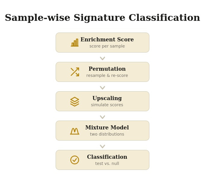
General workflow.
The statistical method is split into 5 steps. Each of those steps is performed for one specific signature at a time. A signature is typically a predefined set of features (transcriptomic expression in this situation) that is associated with some biological state, pathway, or phenotype.
Step 1. Enrichment score
The enrichment scores are first computed for every single sample with the Bioconductor GSVA package (Hänzelmann et al. 2013). Those scores represent the real score for each sample. Later steps treat this real score as the anchor point around which uncertainty gets modeled.
Step 2. Permutation
Random subsets of samples, of fixed size, from the full dataset are repeatedly drawn. For each of these resampled subsets, the enrichment score for the samples present is recomputed.
This step enables a per-sample uncertainty estimation (standard deviation).
Step 3. Upscaling
For each sample, a fixed number of simulated enrichment scores are drawn from a normal distribution centered on the real score, using the standard deviation estimated from permutations.
This step enables the upscaling of the total number of values that will be used in the next step.
Step 4. Mixture model
The synthetic values across all samples are pooled to fit two overlapping normal distributions to them. The two normal distributions are extracted using a mixture model approach implemented in the mixtools package (Benaglia et al. 2009). The assumption is that the whole cohort is a blend of two underlying populations (a “low-mean” population and a “high-mean” population).
Step 5. Classification
Each sample is classified with a one-sided hypothesis test based on the “low-mean” distribution of the mixture model (from Step 4):
- Null hypothesis (H₀): the sample belongs to the “low-mean” distribution
- Alternative hypothesis (H₁): the sample belongs to the “high-mean” distribution
The 95th percentile of the “low-mean” distribution is used as the classification threshold. Each sample’s real enrichment score (from Step 1) is compared to this threshold. A score above the threshold has less than a 5% probability of being produced by the “low-mean” distribution (one-sided p-value < 0.05). In that case, H₀ is rejected.
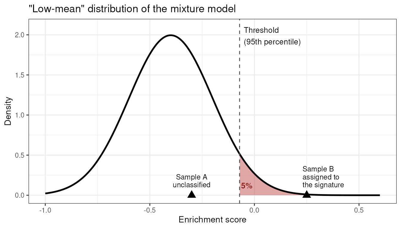
Classification of the samples (schematic). The curve represents the “low-mean” distribution of the mixture model. The dashed line is the classification threshold (95th percentile) and the shaded area represents the upper 5% of the distribution. Sample A, with a score below the threshold, remains unclassified while sample B, with a score above the threshold, is assigned to the signature.
When H₀ is rejected (p-value < 0.05), the sample is assigned to the tested signature. Otherwise, the sample is labeled as “unclassified” for that signature.
Since each signature is tested independently, a sample can be assigned to one signature, to several signatures, or to none of them.
Available signatures
The splitTypeR package provides transcriptomic signatures.
The getGeneSignaturesNames() function lists the names of all the available signatures.
## List the names of the available signatures
getGeneSignaturesNames()
## [1] "Tiriac_PDAC_PDO_Basal_like" "Tiriac_PDAC_PDO_Classical"
## [3] "Moffitt_Basal_like" "Moffitt_Classical"
## [5] "Miyabayashi_Fast" "Miyabayashi_Slow"The getGenesInSignature() function returns the genes of one signature, while the getGeneSignatures() function returns a named list containing one or more signatures. When no name is given, getGeneSignatures() returns all the available signatures.
## Get the genes of the basal-like signature
getGenesInSignature(name="Tiriac_PDAC_PDO_Basal_like")
## [1] "ANO1" "ADORA2B" "S100A2" "CSF2" "ANXA1" "EREG"
## [7] "RGS20" "CELSR1" "WNT7B" "AMIGO2" "PTHLH" "C12orf54"
## [13] "TGM2" "REEP3" "DCBLD2" "NMB" "IKZF2" "GPR87"
## [19] "MUC16" "IVL" "SPRR1B" "BCAR3" "TTC9" "PTGES"
## [25] "CST6" "CATSPER1"
## Get all the available signatures and count the genes in each one
allSignatures <- getGeneSignatures()
lengths(allSignatures)## Tiriac_PDAC_PDO_Basal_like Tiriac_PDAC_PDO_Classical
## 26 62
## Moffitt_Basal_like Moffitt_Classical
## 25 25
## Miyabayashi_Fast Miyabayashi_Slow
## 231 333The current signatures are:
- Tiriac_PDAC_PDO_Basal_like: the basal-like signature (26 genes) defined for pancreatic ductal adenocarcinoma (PDAC) patient-derived organoids (PDOs) in Tiriac et al. (Tiriac et al. 2018).
- Tiriac_PDAC_PDO_Classical: the classical signature (62 genes) defined for PDAC PDOs in Tiriac et al. (Tiriac et al. 2018).
- Moffitt_Basal_like: the original basal-like signature (25 genes) defined for PDAC in Moffitt et al. (Moffitt et al. 2015).
- Moffitt_Classical: the original classical signature (25 genes) defined for PDAC in Moffitt et al. (Moffitt et al. 2015).
- Miyabayashi_Fast: the fast signature (231 genes), updated from the Ensembl IDs (GENCODE v48/org.Hs.eg.db), defined for PDAC xenografts in Miyabayashi et al. (Miyabayashi et al. 2020).
- Miyabayashi_Slow: the slow signature (333 genes), updated from the Ensembl IDs (GENCODE v48/org.Hs.eg.db), defined for PDAC xenografts in Miyabayashi et al. (Miyabayashi et al. 2020).
Using your own signatures
The method is not limited to the signatures included in the
splitTypeR package. Any named
list of at least two gene vectors can be passed to the
runSubtypingBimodal() function. The names of the list are used
as the signature names in the results. The gene identifiers must use the
same format as the row names of the expression matrix (e.g., gene names,
Ensembl IDs). Genes absent from the expression matrix are ignored. It is
recommended to use signatures with 10 genes or more to ensure
statistical stability and reliability of the enrichment scores.
## Example of custom signatures
mySignatures <- list(
SignatureA=c("GENE1", "GENE2", "GENE3", "GENE4", "GENE5", "GENE6",
"GENE7", "GENE8", "GENE9", "GENE10", "GENE11"),
SignatureB=c("GENE4", "GENE9", "GENE10", "GENE12", "GENE13", "GENE15",
"GENE16", "GENE17", "GENE18", "GENE19", "GENE20", "GENE21"))Demonstration
For this demonstration, we are going to use the published RNA-seq dataset of pancreatic ductal adenocarcinoma (PDAC) patient-derived organoids (PDOs) published in Tiriac et al. (Tiriac et al. 2018). The RNA-seq has been aligned with GENCODE v48 on GRCh38.p14 genome with STAR v2.7.9a (Dobin et al. 2013). Only one PDO per patient was retained. The expected counts were processed with DESeq2 v1.50.2 (Love et al. 2014) on genes expressed in at least 20% of the PDOs. The normalized expression is available in a SummarizedExperiment object.
In PDAC, the basal-like and classical subtypes, as defined in Moffitt et al. (Moffitt et al. 2015), are the two consistently employed molecular subtypes. The classical signature is associated with better prognosis and better response to standard chemotherapy, while the basal-like subtype is associated with worse overall prognosis (Moffitt et al. 2015; O’Kane et al. 2020). These signatures were later redefined for patient-derived organoids (Tiriac et al. 2018).
Prepare the signatures
The basal-like and classical gene signatures used in the demonstration are the ones defined for PDOs in Tiriac et al. (Tiriac et al. 2018).
## Required package
library(splitTypeR)
## Prepare the PDOs basal-like and classical signatures
signaturesList <- list()
signaturesList[["Basal-like"]] <-
getGenesInSignature("Tiriac_PDAC_PDO_Basal_like")
signaturesList[["Classical"]] <-
getGenesInSignature("Tiriac_PDAC_PDO_Classical")Prepare the log2-transformed normalized expected counts
A matrix of normalized expected counts is required. The rows are the genes, while the patients (samples) are the columns.
The row annotation must correspond to the signature format. As an example, if the signatures are composed of gene names, the row annotation for the normalized expected counts must also be gene names.
For GSVA analysis, the normalized expected counts should be log-transformed to enable the use of the Gaussian distribution function. The current behavior of GSVA is to automatically choose one of the available distribution functions.
## Required package
library(SummarizedExperiment)
## Load the SummarizedExperiment object
path <- system.file("extdata", "Tiriac_NormExpCounts.RDS",
package="splitTypeR")
se <- readRDS(path)
## Extract the normalized counts and assign the gene names as row names
## The row names should correspond to the information present in the
## gene signatures. In this case, the gene names are used.
normCounts <- assays(se)[["normalizedCounts"]]
rownames(normCounts) <- rowRanges(se)$gene_name
## Log2-transform the data, adding a small pseudo-count to
## prevent log2(0) errors
log2normCounts <- log2(normCounts + 1)Run the subtyping method
The runSubtypingBimodal function runs all the steps. Three parameters control the permutation and upscaling steps:
| Parameter | Description | Default | Trade-off |
|---|---|---|---|
permRatio |
Proportion of the samples randomly selected in each permutation (Step 2). Must be between 0 and 1, and must not select all the samples. | 0.75 | A lower value creates more variation between permutations, but each GSVA score is computed on fewer samples. |
permNbr |
Number of permutations (Step 2). Must be 5 or higher. | 20 | More permutations give a more stable standard deviation for each sample, but take longer to run since GSVA is run once per permutation. |
upscaleNbr |
Number of values drawn from the normal distribution of each sample (Step 3). Must be 2 or higher. | 10 | More values give more data to fit the mixture model (Step 4), with little impact on the run time. |
Each sample is present, on average, in permRatio ×
permNbr permutations (15 with the default values), which is
the number of values used to estimate its standard deviation.
## Fix seed for reproducible results
set.seed(81)
## Run the subtyping method using the log2-transformed data
result <- runSubtypingBimodal(geneLists=signaturesList,
expectedCountsMatrixLog=log2normCounts,
permRatio=0.75,
permNbr=20,
upscaleNbr=12)
## Summary of the classification results
result## A SplitTypeRdata object
## Signatures (2): Basal-like (26 genes), Classical (62 genes)
## Samples: 39
## Completed steps: gsvaResults, permutations, standardDeviation, upscaling, model, threshold, classification
## Classification:
## Basal-like: 13 assigned, 26 unclassified
## Classical: 27 assigned, 12 unclassified
## Use classification() to get the classification of each sample.The resulting object contains information from each step of the process. The information can be accessed using the appropriate getter function.
## Get the list of genes in the classical signature
signatures(result)[["Classical"]]## [1] "MUC13" "GPR35" "USH1C" "BAIAP2L2" "GAL3ST1"
## [6] "VIL1" "DDC" "LGALS4" "TSPAN8" "SLC5A1"
## [11] "SEMA4G" "TNFRSF11A" "HSD17B2" "CKMT1A" "DPCR1"
## [16] "GCNT3" "SLC6A20" "POF1B" "NR1I2" "MUC17"
## [21] "HHLA2" "BTNL8" "HEPH" "PDZD3" "MYO1A"
## [26] "CDH17" "MYO7B" "GPA33" "CALML4" "ANXA13"
## [31] "TM4SF20" "SI" "SLC44A4" "FAM83E" "SLC40A1"
## [36] "CTSE" "BACE2" "SULT1C2" "AGR3" "ATP7B"
## [41] "LYZ" "TESC" "TOX3" "SH3BGRL2" "GMDS"
## [46] "GATA6" "GPX2" "CA2" "ST6GALNAC1" "FOXA3"
## [51] "AKR1C3" "TMC5" "CYP2S1" "PAQR8" "HKDC1"
## [56] "IYD" "DOK4" "CYP2C18" "KCNE3" "FZD5"
## [61] "RASEF" "GKN1"
## Get the GSVA scores for all samples in each signature
gsvaResults(result)## hF2 hF23 hF24 hF27 hF28 hF3
## Basal-like 0.9318280 -0.03854167 -0.2301837 0.1225434 0.5857513 0.9833333
## Classical -0.9134078 0.10297767 0.2214765 -0.1309421 -0.5614173 -0.9829707
## hF31 hF32 hF34 hF39 hF43 hF44
## Basal-like -0.4769812 -0.3051282 -0.5843797 -0.4853994 -0.2838235 -0.7680835
## Classical 0.4431077 0.2409733 0.3870926 0.4834900 0.1909814 0.6826443
## hF50 hF57 hM17D hM19A hM1A hM8
## Basal-like 0.3194667 -0.8285276 -0.1657321 0.8758845 0.5039683 0.9084949
## Classical -0.2185772 0.7852966 0.1781993 -0.8022948 -0.4360974 -0.7763975
## hT1 hT101 hT102 hT105 hT108 hT123
## Basal-like 0.4552901 -0.0738573 -0.7361761 0.2980769 -0.1111111 -0.2083333
## Classical -0.3147877 0.1204267 0.6841604 -0.3511774 0.1682968 0.2387448
## hT125 hT127 hT25 hT3 hT30 hT48
## Basal-like 0.3246225 0.804817 -0.4921797 -0.8297218 -0.3125731 0.12342611
## Classical -0.2855204 -0.718669 0.3966346 0.7642829 0.2075656 -0.06132129
## hT60 hT81 hT82 hT85 hT89 hT91
## Basal-like 0.9600173 -0.4809993 0.6633929 -0.950000 -0.3759857 -0.9194444
## Classical -0.9035783 0.4877874 -0.5354225 0.941871 0.3297384 0.8405669
## hT93 hT96 hT98
## Basal-like -0.5982201 -0.3102627 -0.2657718
## Classical 0.5818909 0.3609801 0.2376757
## attr(,"gsvaParam")
## attr(,"gsvaParam")$originalClassWasSE
## [1] FALSE
##
## attr(,"gsvaParam")$geneSets
## attr(,"gsvaParam")$geneSets$`Basal-like`
##  [1] "ANO1"     "ADORA2B"  "S100A2"   "CSF2"     "ANXA1"    "EREG"
##  [7] "RGS20"    "CELSR1"   "WNT7B"    "AMIGO2"   "PTHLH"    "C12orf54"
## [13] "TGM2"     "REEP3"    "DCBLD2"   "NMB"      "IKZF2"    "GPR87"
## [19] "MUC16"    "IVL"      "SPRR1B"   "BCAR3"    "TTC9"     "PTGES"
## [25] "CST6"     "CATSPER1"
##
## attr(,"gsvaParam")$geneSets$Classical
##  [1] "MUC13"      "GPR35"      "USH1C"      "BAIAP2L2"   "GAL3ST1"
##  [6] "VIL1"       "DDC"        "LGALS4"     "TSPAN8"     "SLC5A1"
## [11] "SEMA4G"     "TNFRSF11A"  "HSD17B2"    "CKMT1A"     "DPCR1"
## [16] "GCNT3"      "SLC6A20"    "POF1B"      "NR1I2"      "MUC17"
## [21] "HHLA2"      "BTNL8"      "HEPH"       "PDZD3"      "MYO1A"
## [26] "CDH17"      "MYO7B"      "GPA33"      "CALML4"     "ANXA13"
## [31] "TM4SF20"    "SI"         "SLC44A4"    "FAM83E"     "SLC40A1"
## [36] "CTSE"       "BACE2"      "SULT1C2"    "AGR3"       "ATP7B"
## [41] "LYZ"        "TESC"       "TOX3"       "SH3BGRL2"   "GMDS"
## [46] "GATA6"      "GPX2"       "CA2"        "ST6GALNAC1" "FOXA3"
## [51] "AKR1C3"     "TMC5"       "CYP2S1"     "PAQR8"      "HKDC1"
## [56] "IYD"        "DOK4"       "CYP2C18"    "KCNE3"      "FZD5"
## [61] "RASEF"      "GKN1"
##
##
## attr(,"gsvaParam")$assay
## [1] NA
##
## attr(,"gsvaParam")$annotation
## geneIdType: Null
##
## attr(,"gsvaParam")$minSize
## [1] 1
##
## attr(,"gsvaParam")$maxSize
## [1] Inf
##
## attr(,"gsvaParam")$nzcount
## [1] 3354
##
## attr(,"gsvaParam")$ondisk
## [1] "auto"
##
## attr(,"gsvaParam")$checkNA
## [1] "auto"
##
## attr(,"gsvaParam")$didCheckNA
## [1] TRUE
##
## attr(,"gsvaParam")$anyNA
## [1] FALSE
##
## attr(,"gsvaParam")$use
## [1] "everything"
##
## attr(,"gsvaParam")$rowNorm
## [1] "ecdf"
##
## attr(,"gsvaParam")$kcdf
## [1] "auto"
##
## attr(,"gsvaParam")$kcdfNoneMinSampleSize
## [1] 200
##
## attr(,"gsvaParam")$tau
## [1] 1
##
## attr(,"gsvaParam")$maxDiff
## [1] TRUE
##
## attr(,"gsvaParam")$absRanking
## [1] FALSE
##
## attr(,"gsvaParam")$sparse
## [1] FALSE
##
## attr(,"gsvaParam")$filterRows
## [1] TRUE
##
## attr(,"assay")
## [1] "es"
## attr(,"gsvaVersion")
## [1] "2.7.25"
## attr(,"geneSets")
## attr(,"geneSets")$`Basal-like`
## [1] "ANO1" "ADORA2B" "S100A2" "CSF2" "ANXA1" "EREG"
## [7] "RGS20" "CELSR1" "WNT7B" "AMIGO2" "PTHLH" "C12orf54"
## [13] "TGM2" "REEP3" "DCBLD2" "NMB" "IKZF2" "GPR87"
## [19] "MUC16" "IVL" "SPRR1B" "BCAR3" "TTC9" "PTGES"
## [25] "CST6" "CATSPER1"
##
## attr(,"geneSets")$Classical
## [1] "MUC13" "GPR35" "USH1C" "BAIAP2L2" "GAL3ST1"
## [6] "VIL1" "DDC" "LGALS4" "TSPAN8" "SLC5A1"
## [11] "SEMA4G" "TNFRSF11A" "HSD17B2" "CKMT1A" "GCNT3"
## [16] "SLC6A20" "POF1B" "NR1I2" "MUC17" "HHLA2"
## [21] "BTNL8" "HEPH" "MYO1A" "CDH17" "MYO7B"
## [26] "GPA33" "CALML4" "ANXA13" "TM4SF20" "SI"
## [31] "SLC44A4" "FAM83E" "SLC40A1" "CTSE" "BACE2"
## [36] "SULT1C2" "AGR3" "ATP7B" "LYZ" "TESC"
## [41] "TOX3" "SH3BGRL2" "GMDS" "GATA6" "GPX2"
## [46] "CA2" "ST6GALNAC1" "FOXA3" "AKR1C3" "TMC5"
## [51] "CYP2S1" "PAQR8" "HKDC1" "IYD" "DOK4"
## [56] "CYP2C18" "KCNE3" "FZD5" "RASEF" "GKN1"
## Get the GSVA scores for the first 5 samples in the first 6 permutations
## (columns) done for the classical signature
permutations(result)[['Classical']][seq_len(5), seq_len(6)]
## [,1] [,2] [,3] [,4] [,5] [,6]
## hF2 -0.87955840 NA -0.87809349 NA -0.91255814 -0.8899771
## hF23 NA -0.08950456 0.23653846 0.04872661 0.22668030 0.0604898
## hF24 NA 0.02841517 0.42270683 0.22947277 0.31273837 0.1506945
## hF27 -0.03941731 -0.20563925 0.01829787 -0.08884449 -0.03654507 NA
## hF28 -0.51596289 NA -0.39893080 -0.49631064 -0.47531573 -0.5683230
## Get the standard deviation of the GSVA scores for all samples for the
## classical signature
## The standard deviation is inferred from the permutation step
standardDeviation(result)$Classical
## hF2 hF23 hF24 hF27 hF28 hF3
## 0.026561380 0.095755725 0.120798797 0.081266938 0.065186429 0.008675902
## hF31 hF32 hF34 hF39 hF43 hF44
## 0.058667114 0.066535776 0.058671052 0.054471237 0.067684116 0.046198986
## hF50 hF57 hM17D hM19A hM1A hM8
## 0.077368473 0.023114593 0.092320169 0.018058727 0.056724043 0.034555804
## hT1 hT101 hT102 hT105 hT108 hT123
## 0.053921809 0.090626892 0.044054124 0.055389871 0.089983704 0.127169294
## hT125 hT127 hT25 hT3 hT30 hT48
## 0.079977292 0.032523448 0.075156258 0.022793985 0.073668955 0.105088007
## hT60 hT81 hT82 hT85 hT89 hT91
## 0.025490655 0.057336766 0.047046295 0.022329616 0.070573879 0.021891698
## hT93 hT96 hT98
## 0.046301231 0.041979712 0.088366419
## Get the first 6 upscaling GSVA scores (columns) for the first 5 samples
## for the classical signature
upscaling(result)[['Classical']][seq_len(5), seq_len(6)]
## [,1] [,2] [,3] [,4] [,5] [,6]
## hF2 -0.8904656 -0.89107386 -0.90166058 -0.90156532 -0.92802494 -0.928665397
## hF23 0.2105585 0.19225589 0.12700464 0.05938685 0.10731097 -0.005661387
## hF24 0.4323339 0.21149687 0.09129895 0.16668457 0.08051689 0.028841760
## hF27 -0.2041871 -0.04549904 -0.03582384 -0.16268045 -0.12812664 -0.130654394
## hF28 -0.3981220 -0.68175972 -0.63945097 -0.41295596 -0.46945658 -0.610334888
## Get the mixture model for the classical signature
## This is a mixEM object
classicalModel <- model(result)[['Classical']]

## Get the two distribution means
classicalModel$mu
## [1] -0.6505149 0.3254568
## Get the two distribution standard deviations
classicalModel$sigma
## [1] 0.2503627 0.3296842
## Get the mixing proportions (the fraction of the values assigned to each
## distribution)
classicalModel$lambda
## [1] 0.2802048 0.7197952
## Get the classification threshold of each signature
## The threshold is the 95th percentile of the "low-mean" distribution
threshold(result)
## $`Basal-like`
## [1] 0.249288
##
## $Classical
## [1] -0.238705
## Get the final classification of the first samples
## for the classical signature
head(classification(result)[['Classical']])
## GSVA_score classification
## hF2 -0.9134078 unclassified
## hF23 0.1029777 Classical
## hF24 0.2214765 Classical
## hF27 -0.1309421 Classical
## hF28 -0.5614173 unclassified
## hF3 -0.9829707 unclassifiedVisual representation of the results at the permutation step
The plotPermutationSamplesDistribution() function enables the visualization of the GSVA results obtained during the permutation step for a specific signature and specific samples.
## The GSVA results obtained for three samples during the permutation step
## for the classical signature
## The seed is fixed to ensure reproducibility
plotPermutationSamplesDistribution(x=result, signature="Classical",
    pointColor="darkorange", alpha=1, samples=c("hF23", "hT82", "hT89"),
    seed=121)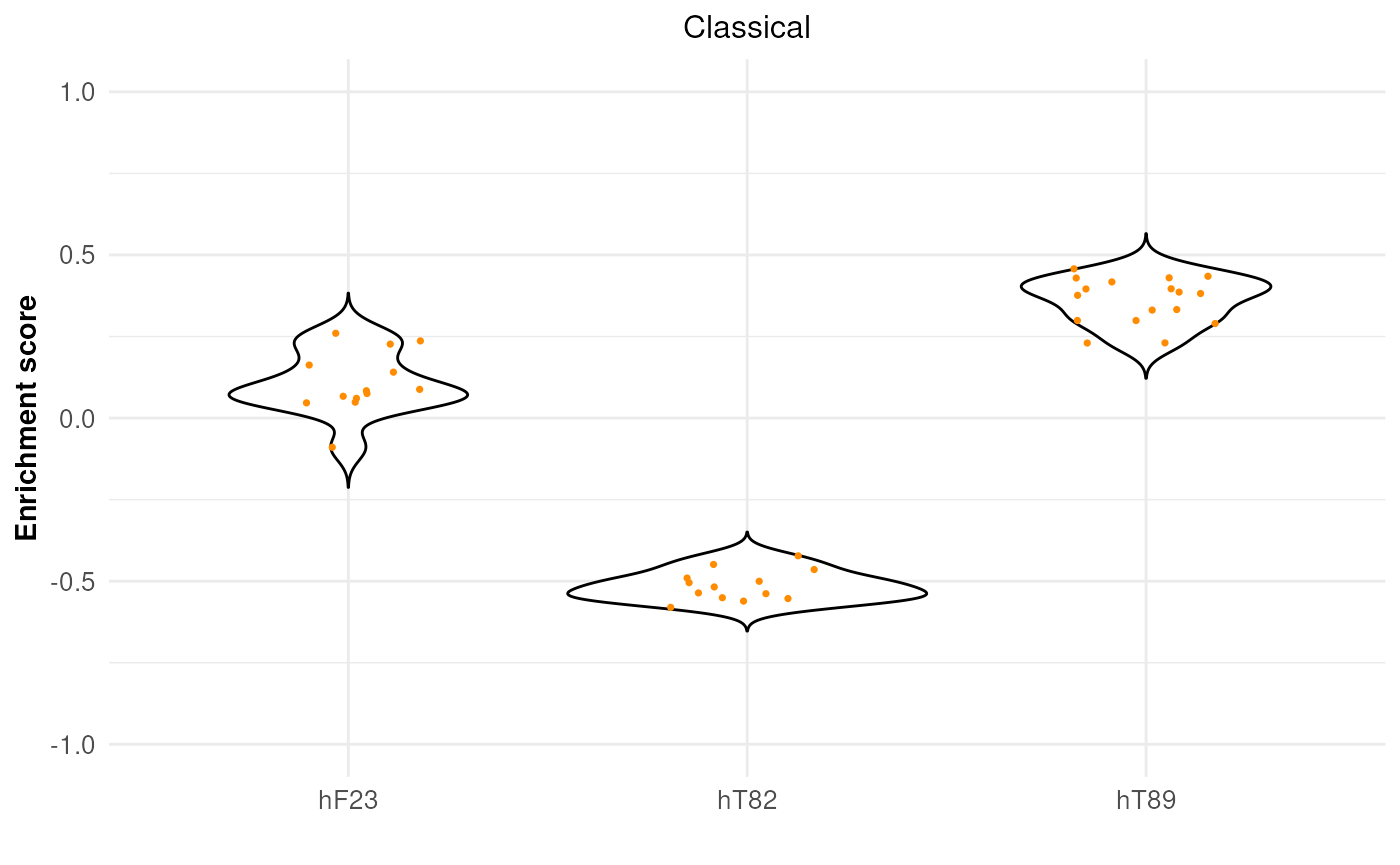
Visual representation of the results at the upscaling step
From the permutation step, the standard deviation is calculated for each sample. The upscaling is done with the real GSVA score as mean and the calculated standard deviation.
The plotPermutationSamplesNormal() function shows the GSVA scores sampled during the upscaling step. The mean is shown as a vertical dotted line, while the normal distribution is shown as a dashed line. The sampled GSVA scores are shown as dots in this graph.
## Fix seed for reproducibility
set.seed(121)

## The GSVA scores sampled for three samples during the upscaling step
## for the classical signature
plotPermutationSamplesNormal(result, signature="Classical",
    samples=c("hF23", "hT82", "hT89"), pointColor="darkviolet")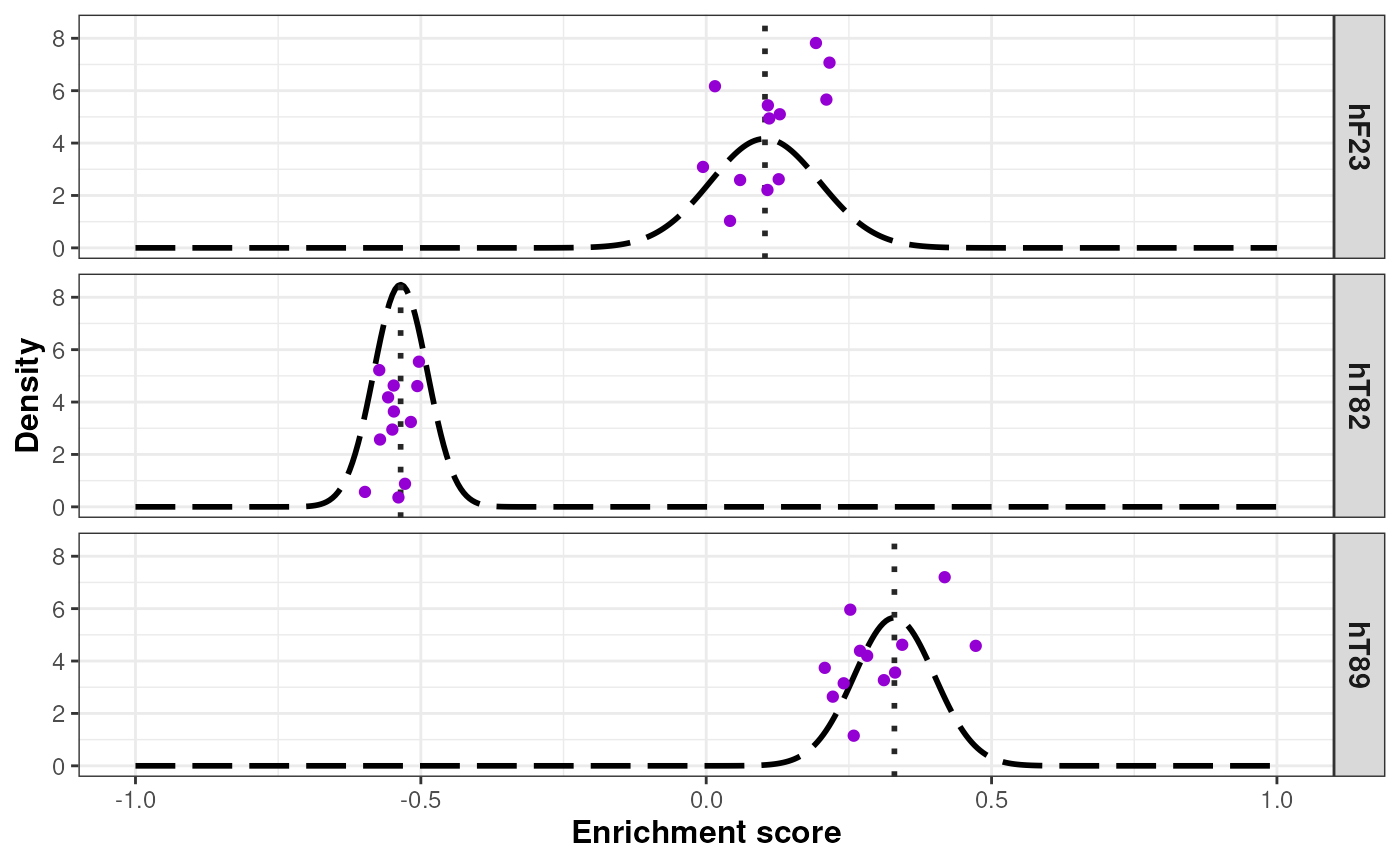
Visual representation of the results at the mixture model step
The plotDensityWithUpscalingSamplesBimodal() function enables the visualization of the two normal distributions obtained for a specific signature. In this graph, the GSVA values are those generated during the upscaling step.
plotDensityWithUpscalingSamplesBimodal(breaks = 26L,
    signature="Basal-like", result)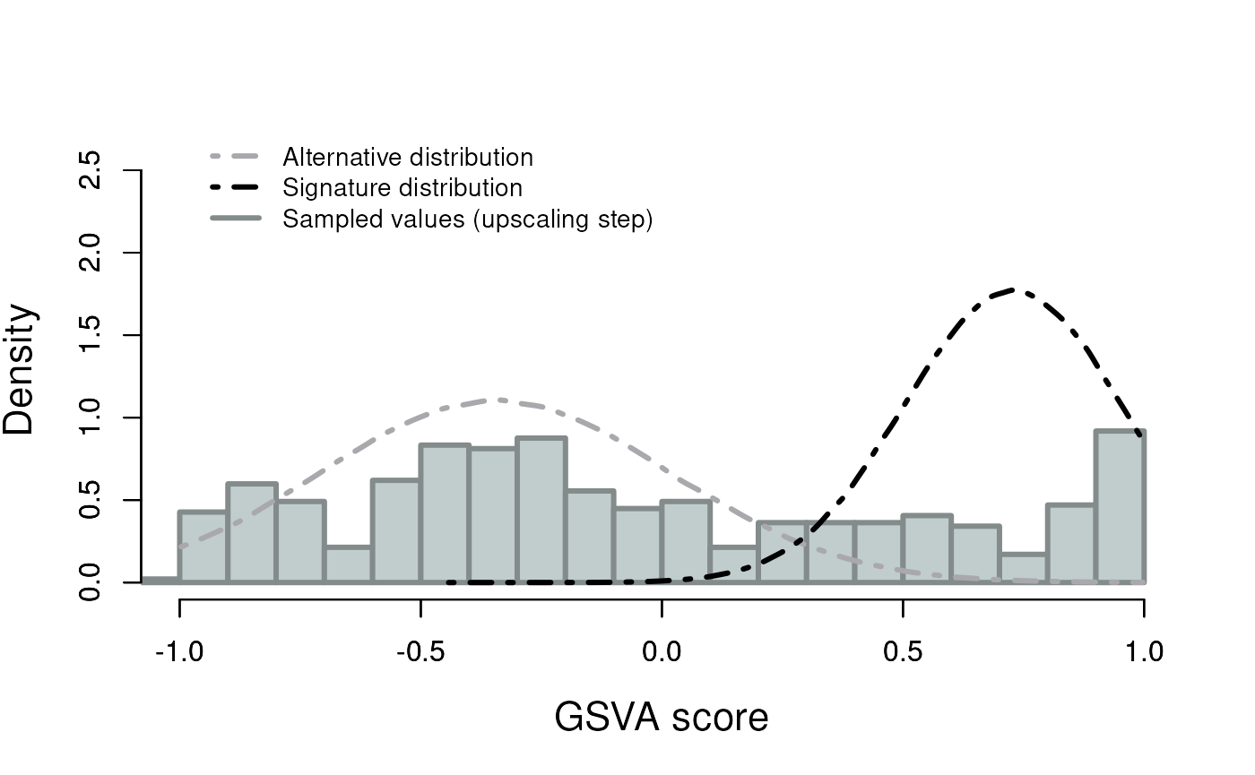
plotDensityWithUpscalingSamplesBimodal(breaks = 26L,
    signature="Classical", result)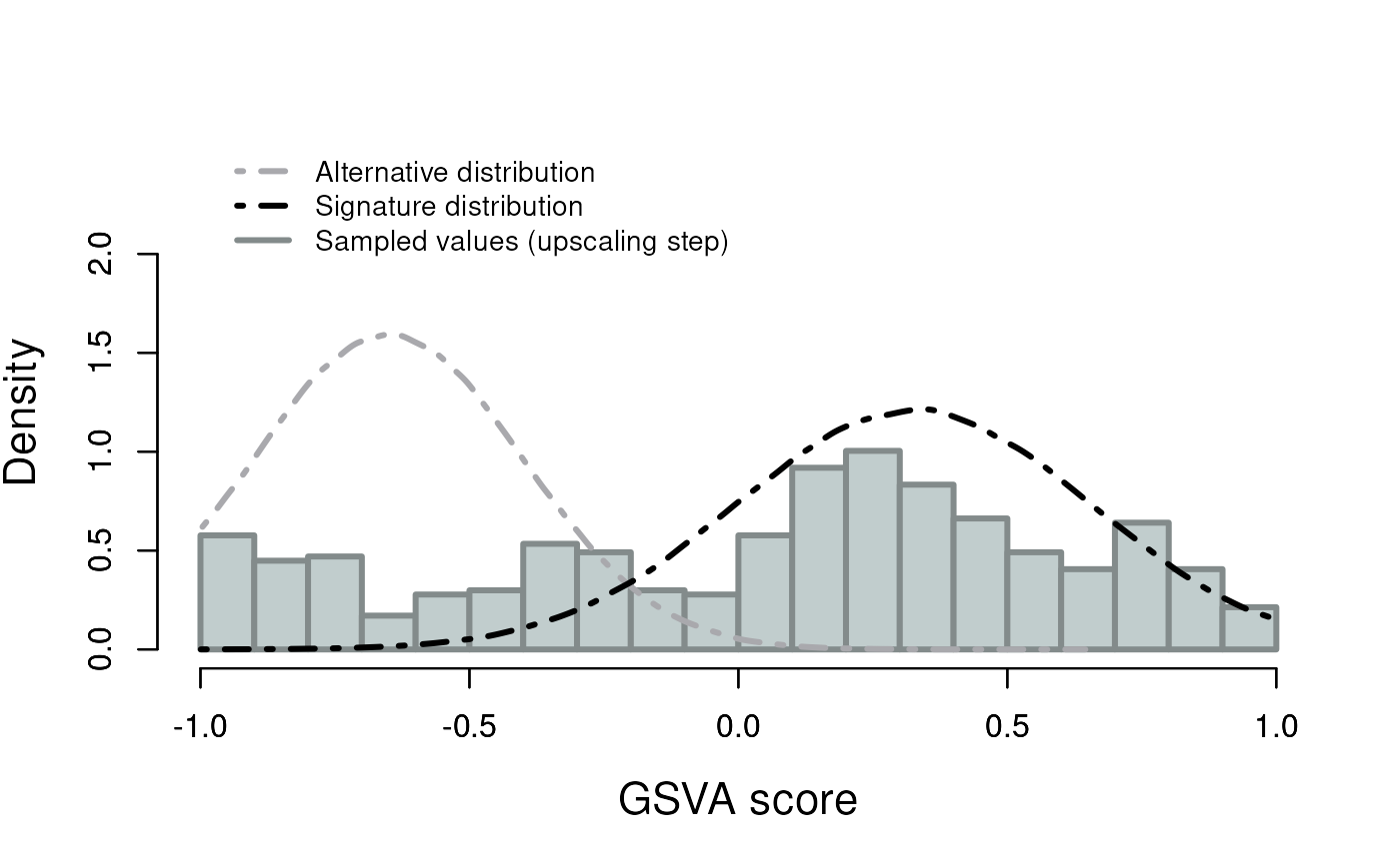
Classification of the samples
Let’s compare the classification obtained here with the one from Tiriac et al. (Tiriac et al. 2018).
## Assignments from Tiriac et al.
pathAssign <- system.file("extdata", "Moffitt_Tiriac_2018_Assignation.txt",
                        package="splitTypeR")
tiriacAssign <- read.table(pathAssign, sep="\t", header=TRUE)

## Assignments from the mixture model are extracted from the result
## By default, the samples are considered unclassified
## The samples are classified only if they are assigned to one of the signatures
## When assigned to both signatures, the samples remain unclassified
assignation <- data.frame(
        Samples=rownames(classification(result)[['Classical']]),
        newAssignation="unclassified")
assignation$Classical <- classification(result)[['Classical']]$classification
assignation$Basal <- classification(result)[['Basal-like']]$classification
assignation$newAssignation[which(assignation$Classical == "Classical" &
                    assignation$Basal == "unclassified")] <- "Classical"
assignation$newAssignation[which(assignation$Basal == "Basal-like" &
                    assignation$Classical == "unclassified")] <- "Basal-like"

## Merge the current assignments with the Tiriac et al. assignments into
## one data frame
assignation <- merge(assignation[, c("Samples", "newAssignation")],
                        tiriacAssign, by.x="Samples",
                        by.y="Line", all.y=FALSE, all.x=FALSE)

table(assignation$newAssignation, assignation$Moffitt)
##
## Basal-like Classical
## Basal-like 8 3
## Classical 1 24
## unclassified 0 1About 86% of the samples (32 out of 37) are assigned the same subtype.
The following graph shows the GSVA scores of each sample for both signatures. The dashed lines represent the classification threshold of each signature (the 95th percentile of the “low-mean” distribution). A sample located to the right of the vertical line is assigned to the classical signature, while a sample located above the horizontal line is assigned to the basal-like signature. The samples for which the classification differs from Tiriac et al. (Tiriac et al. 2018) are labeled.
## Required package
library(ggplot2)

## Get the GSVA score of each sample for both signatures
gsva <- data.frame(
    Samples=rownames(classification(result)[['Classical']]),
    Classical=classification(result)[['Classical']]$GSVA_score,
    Basal=classification(result)[['Basal-like']]$GSVA_score)

## Add the assignments and identify the samples with a different
## classification than Tiriac et al.
gsva <- merge(gsva, assignation, by="Samples")
gsva$Agreement <- ifelse(gsva$newAssignation == gsva$Moffitt,
    "Same classification", "Different classification")

## Classification threshold of each signature
thresholdClassical <- threshold(result)[['Classical']]
thresholdBasal <- threshold(result)[['Basal-like']]

## Scatter plot of the GSVA scores with the classification thresholds
## The vertical dashed line is the classical threshold and the horizontal
## dashed line is the basal-like threshold
ggplot(gsva, aes(x=Classical, y=Basal)) +
    geom_vline(xintercept=thresholdClassical, linetype="dashed",
        color="gray40") +
    geom_hline(yintercept=thresholdBasal, linetype="dashed",
        color="gray40") +
    geom_point(aes(color=Agreement, shape=Moffitt), size=3) +
    geom_text(data=gsva[gsva$Agreement == "Different classification", ],
        aes(label=Samples), vjust=-1, size=3.5) +
    scale_color_manual(values=c("Same classification"="gray60",
        "Different classification"="firebrick")) +
    labs(x="GSVA score - Classical signature",
        y="GSVA score - Basal-like signature",
        color="Compared to Tiriac et al.", shape="Tiriac et al.") +
    theme_bw()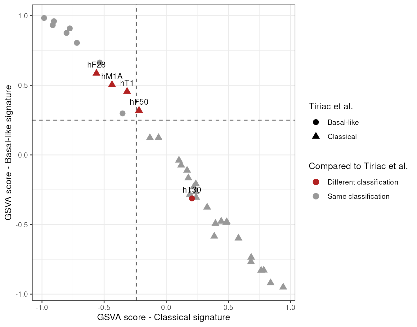
Most samples that are not assigned to the same subtype have intermediate scores and are located where the classical and basal-like samples meet. Sample hF50 is located in the region where both signatures are assigned and therefore remains unclassified.
Acknowledgment
D.A. Tuveson is a distinguished scholar of the Lustgarten Foundation and Director of the Lustgarten Foundation-designated Laboratory of Pancreatic Cancer Research. This project is supported by the Lustgarten Foundation.
Claude Sonnet 5 was used for improving the workflow figure. It was also used for proofreading and copyediting sections of this text.
Claude Opus 5.5, through Claude Code, was used to assist with code maintenance, including renaming the demonstration signatures, updating the associated documentation and unit tests, removing unused internal data, and adding the Quick start section to this vignette. All changes were reviewed and validated by the package maintainer.
Session info
Here is the output of sessionInfo() on the system on
which this document was compiled:
## R Under development (unstable) (2026-10-22 r90748)
## Platform: x86_64-pc-linux-gnu
## Running under: Ubuntu 24.04.4 LTS
##
## Matrix products: default
## BLAS:   /usr/lib/x86_64-linux-gnu/openblas-pthread/libblas.so.3
## LAPACK: /usr/lib/x86_64-linux-gnu/openblas-pthread/libopenblasp-r0.3.26.so;  LAPACK version 3.12.0
##
## locale:
##  [1] LC_CTYPE=en_US.UTF-8       LC_NUMERIC=C
##  [3] LC_TIME=en_US.UTF-8        LC_COLLATE=en_US.UTF-8
##  [5] LC_MONETARY=en_US.UTF-8    LC_MESSAGES=en_US.UTF-8
##  [7] LC_PAPER=en_US.UTF-8       LC_NAME=C
##  [9] LC_ADDRESS=C               LC_TELEPHONE=C
## [11] LC_MEASUREMENT=en_US.UTF-8 LC_IDENTIFICATION=C
##
## time zone: UTC
## tzcode source: system (glibc)
##
## attached base packages:
## [1] stats4    stats     graphics  grDevices utils     datasets  methods
## [8] base
##
## other attached packages:
##  [1] ggplot2_4.0.3               splitTypeR_0.99.8
##  [3] SummarizedExperiment_1.43.0 Biobase_2.73.2
##  [5] GenomicRanges_1.65.4        Seqinfo_1.3.2
##  [7] IRanges_2.47.5              S4Vectors_0.51.10
##  [9] BiocGenerics_0.59.12        generics_0.1.4
## [11] MatrixGenerics_1.25.0       matrixStats_1.5.0
## [13] knitr_1.52                  BiocStyle_2.41.0
##
## loaded via a namespace (and not attached):
##   [1] DBI_1.3.0                   GSEABase_1.75.0
##   [3] rlang_1.3.0                 magrittr_2.0.5
##   [5] otel_0.2.0                  compiler_4.7.0
##   [7] RSQLite_3.53.3              DelayedMatrixStats_1.35.0
##   [9] png_0.1-9                   systemfonts_1.3.2
##  [11] vctrs_0.7.3                 stringr_1.6.0
##  [13] pkgconfig_2.0.3             SpatialExperiment_1.23.0
##  [15] crayon_1.5.3                memuse_4.2-3
##  [17] fastmap_1.2.0               magick_2.9.1
##  [19] XVector_0.53.0              labeling_0.4.3
##  [21] rmarkdown_2.32              graph_1.91.0
##  [23] ragg_1.5.2                  purrr_1.2.2
##  [25] bit_4.6.0                   xfun_0.62
##  [27] cachem_1.1.0                jsonlite_2.0.0
##  [29] blob_1.3.0                  rhdf5filters_1.25.4
##  [31] DelayedArray_0.39.8         Rhdf5lib_2.1.0
##  [33] BiocParallel_1.47.0         parallel_4.7.0
##  [35] R6_2.6.1                    stringi_1.8.9
##  [37] bslib_0.12.0                RColorBrewer_1.1-3
##  [39] jquerylib_0.1.4             Rcpp_1.1.2
##  [41] bookdown_0.48               GSVA_2.7.25
##  [43] mixtools_2.0.0.1            BiocBaseUtils_1.15.1
##  [45] Matrix_1.7-6                splines_4.7.0
##  [47] tidyselect_1.2.1            abind_1.4-8
##  [49] yaml_2.3.12                 codetools_0.2-20
##  [51] lattice_0.23-1              tibble_3.3.1
##  [53] withr_3.0.3                 KEGGREST_1.53.6
##  [55] S7_0.2.2                    evaluate_1.0.5
##  [57] survival_3.8-12             desc_1.4.3
##  [59] kernlab_0.9-33              Biostrings_2.81.9
##  [61] pillar_1.11.1               BiocManager_1.30.27
##  [63] plotly_4.12.1               sparseMatrixStats_1.25.0
##  [65] scales_1.4.0                xtable_1.8-8
##  [67] glue_1.8.1                  tools_4.7.0
##  [69] data.table_1.18.6.1         annotate_1.91.0
##  [71] fs_2.1.0                    XML_3.99-0.25
##  [73] rhdf5_2.57.20               grid_4.7.0
##  [75] tidyr_1.3.2                 AnnotationDbi_1.75.2
##  [77] SingleCellExperiment_1.35.2 nlme_3.1-171
##  [79] HDF5Array_1.41.3            cli_3.6.6
##  [81] textshaping_1.0.5           segmented_2.2-2
##  [83] S4Arrays_1.13.2             viridisLite_0.4.3
##  [85] dplyr_1.2.1                 gtable_0.3.6
##  [87] sass_0.4.10                 digest_0.6.39
##  [89] SparseArray_1.13.4          rjson_0.2.23
##  [91] htmlwidgets_1.6.4           farver_2.1.2
##  [93] memoise_2.0.1               htmltools_0.5.9
##  [95] pkgdown_2.2.0               lifecycle_1.0.5
##  [97] h5mread_1.5.3               httr_1.4.9
##  [99] MASS_7.3-66                 bit64_4.8.6