Robust Ancestry Inference using Data Synthesis
Pascal Belleau, Astrid Deschênes and Alexander Krasnitz
Source:vignettes/RAIDS.Rmd
RAIDS.Rmd
Package: RAIDS
Authors: Pascal Belleau [cre, aut] (ORCID: https://orcid.org/0000-0002-0802-1071), Astrid Deschênes
[aut] (ORCID: https://orcid.org/0000-0001-7846-6749), David A. Tuveson
[aut] (ORCID: https://orcid.org/0000-0002-8017-2712), Alexander
Krasnitz [aut]
Version: 1.7.3
Compiled date: 2025-10-08
License: Apache License (>= 2)
Licensing
The RAIDS
package and the underlying RAIDS code are
distributed under
the https://opensource.org/licenses/Apache-2.0 license. You
are free to use and redistribute this software.
Citing
If you use the RAIDS package for a publication, we would ask you to cite the following:
Pascal Belleau, Astrid Deschênes, Nyasha Chambwe, David A. Tuveson, Alexander Krasnitz; Genetic Ancestry Inference from Cancer-Derived Molecular Data across Genomic and Transcriptomic Platforms. Cancer Res 1 January 2023; 83 (1): 49–58. https://doi.org/10.1158/0008-5472.CAN-22-0682
Introduction
The RAIDS (Robust Ancerstry Inference using Data Synthesis) package enables accurate and robust inference of genetic ancestry from human molecular data other than whole-genome or whole-exome sequences of cancer-free DNA. The current version can handle sequences of:
- whole genomes
- whole exomes
- targeted gene panels
- RNA,
including those from cancer-derived nucleic acids. The RAIDS package implements a data synthesis method that, for any given molecular profile of an idividual, enables, on the one hand, profile-specific inference parameter optimization and, on the other hand, a profile-specific inference accuracy estimate. By the molecular profile we mean a table of the individual’s germline genotypes at genome positions with sufficient read coverage in the individual’s input data, where sequence variants are frequent in the population reference data.
Installation
To install this package from Bioconductor, start R (version 4.3 or later) and enter:
if (!requireNamespace("BiocManager", quietly = TRUE))
        install.packages("BiocManager")

BiocManager::install("RAIDS")
Using RAIDS: step-by-step explanation
This is an overview of the RAIDS inferential framework:
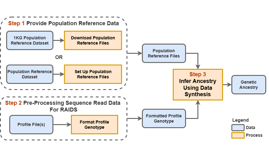
An overview of the genetic ancestry inference procedure.
The main steps are:
Step 1. Set-up working directory and provide population reference files
Step 2 Sample the reference data for donors whose genotypes will be used for synthesis and optimize ancestry inference parameters using synthetic data
Step 3 Infer ancestry
Step 4 Summarize and visualize the results
These steps are described in detail in the following.
Step 1. Set-up working directory and provide population reference files
1.1 Create a working directory structure
First, the following working directory structure should be created:
#############################################################################
## Working directory structure
#############################################################################
workingDirectory/
    data/
        refGDS
        profileGDS
The following code creates a temporary working directory structure where the example will be run.
#############################################################################
## Create a temporary working directory structure
##    using the tempdir() function
#############################################################################
pathWorkingDirectory <- file.path(tempdir(), "workingDirectory")
pathWorkingDirectoryData <- file.path(pathWorkingDirectory, "data")

if (!dir.exists(pathWorkingDirectory)) {
        dir.create(pathWorkingDirectory)
        dir.create(pathWorkingDirectoryData)
        dir.create(file.path(pathWorkingDirectoryData, "refGDS"))
        dir.create(file.path(pathWorkingDirectoryData, "profileGDS"))
}
1.2 Download the population reference files
The population reference files should be downloaded into the data/refGDS sub-directory. This following code downloads the complete pre-processed files for 1000 Genomes (1KG), for the hg38 build of the human genome, in the GDS format. The size of the 1KG GDS file is 15GB.
#############################################################################
## How to download the pre-processed files for 1000 Genomes (1KG) (15 GB)
#############################################################################
cd workingDirectory
cd data/refGDS

wget https://labshare.cshl.edu/shares/krasnitzlab/aicsPaper/matGeno1000g.gds
wget https://labshare.cshl.edu/shares/krasnitzlab/aicsPaper/matAnnot1000g.gds
cd -
For illustrative purposes, a small population reference GDS file (called ex1_good_small_1KG.gds) and a small population reference SNV Annotation GDS file (called ex1_good_small_1KG_Annot.gds) are included in this package. Please note that these “mini-reference” files are for illustrative purposes only and cannot be used to infer genetic ancestry reliably.
In this example, the mini-reference files are copied to the data/refGDS directory.
#############################################################################
## Load RAIDS package
#############################################################################
library(RAIDS)

#############################################################################
## The population reference GDS file and SNV Annotation GDS file
##    need to be located in the same sub-directory.
## Note that the mini-reference GDS file used for this example is
##    NOT sufficient for reliable inference.
#############################################################################
## Path to the demo 1KG GDS file is located in this package
dataDir <- system.file("extdata", package="RAIDS")
pathReference <- file.path(dataDir, "tests")

fileGDS <- file.path(pathReference, "ex1_good_small_1KG.gds")
fileAnnotGDS <- file.path(pathReference, "ex1_good_small_1KG_Annot.gds")

file.copy(fileGDS, file.path(pathWorkingDirectoryData, "refGDS"))
## [1] TRUE
file.copy(fileAnnotGDS, file.path(pathWorkingDirectoryData, "refGDS"))
## [1] TRUE
Step 2 Ancestry inference with RAIDS
2.1 Set-up the required directories
All required directories are created at this point. In addition, the paths to the reference files are stored in variables for later use.
#############################################################################
## The file path to the population reference GDS file
##     is required (refGenotype will be used as input later)
## The file path to the population reference SNV Annotation GDS file
##     is also required (refAnnotation will be used as input later)
#############################################################################
pathReference <- file.path(pathWorkingDirectoryData, "refGDS")

refGenotype <- file.path(pathReference, "ex1_good_small_1KG.gds")
refAnnotation <- file.path(pathReference, "ex1_good_small_1KG_Annot.gds")

#############################################################################
## The output profileGDS directory, inside workingDirectory/data, must be
##    created (pathProfileGDS will be used as input later)
#############################################################################
pathProfileGDS <- file.path(pathWorkingDirectoryData, "profileGDS")

if (!dir.exists(pathProfileGDS)) {
    dir.create(pathProfileGDS)
}
2.2 Sample the reference data for donors whose genotypes will be used for synthesis and optimize ancestry inference parameters using synthetic data
With the 1KG reference, we recommend sampling 30 donor profiles per sub-continental population. For reproducibility, be sure to use the same random-number generator seed.
In the following code, only 2 individual profiles per sub-continental population are sampled from the demo population GDS file:
#############################################################################
## Set up the following random number generator seed to reproduce
##    the expected results
#############################################################################
set.seed(3043)

#############################################################################
## Choose the profiles from the population reference GDS file for
##   data synthesis.
## Here we choose 2 profiles per subcontinental population
##   from the mini 1KG GDS file.
## Normally, we would use 30 randomly chosen profiles per
##   subcontinental population.
#############################################################################
dataRef <- select1KGPopForSynthetic(fileReferenceGDS=refGenotype,
                                        nbProfiles=2L)
2.3 Infer ancestry
Within a single function call, data synthesis is performed, the synthetic data are used to optimize the inference parameters and, with these, the ancestry is inferred from the input sequence profile.
According to the type of input data (RNA or DNA sequence), a specific function should be called. The inferAncestry() function (inferAncestryDNA() is the same as inferAncestry() ) is used for DNA profiles while the inferAncestryGeneAware() function is RNA specific.
The inferAncestry() function requires a specific input format for the individual’s genotyping profile as explained in the Introduction. The format is set by the genoSource parameter.
One of the allowed formats is VCF (genoSource=c(“VCF”)), with the following mandatory fields: GT, AD and DP. The VCF file must be gzipped.
Also allowed is a “generic” file format (genoSource=c(“generic”)), specified as a comma-separated table The following columns are mandatory:
- Chromosome: The name of the chromosome can be formatted as chr1 or 1
- Position: The position on the chromosome
- Ref: The reference nucleotide
- Alt: The alternative nucleotide
- Count: The total read count
- File1R: Read count for the reference nucleotide
- File1A: Read count for the alternative nucleotide
Note: a header with identical column names is required.
In this example, the profile is from DNA source and requires the use of the inferAncestry() function.
###########################################################################
## Seqinfo and BSgenome are required libraries to run this example
###########################################################################
if (requireNamespace("Seqinfo", quietly=TRUE) &&
      requireNamespace("BSgenome.Hsapiens.UCSC.hg38", quietly=TRUE)) {

    #######################################################################
    ## Chromosome length information is required
    ## chr23 is chrX, chr24 is chrY and chrM is 25
    #######################################################################
    genome <- BSgenome.Hsapiens.UCSC.hg38::Hsapiens
    chrInfo <- Seqinfo::seqlengths(genome)[1:25]

    #######################################################################
    ## The demo SNP VCF file of the DNA profile donor
    #######################################################################
    fileDonorVCF <- file.path(dataDir, "example", "snpPileup", "ex1.vcf.gz")

    #######################################################################
    ## The ancestry inference call
    #######################################################################
    resOut <- inferAncestry(profileFile=fileDonorVCF,
        pathProfileGDS=pathProfileGDS,
        fileReferenceGDS=refGenotype,
        fileReferenceAnnotGDS=refAnnotation,
        chrInfo=chrInfo,
        syntheticRefDF=dataRef,
        genoSource=c("VCF"))
}
The temporary files created in this example are deleted as follows.
#######################################################################
## Remove temporary files created for this demo
#######################################################################
unlink(pathWorkingDirectory, recursive=TRUE, force=TRUE)
Step 3. Examine the value of the inference call
The inferred ancestry and the optimal parameters are present in the list object generated by the inferAncestry() and inferAncestryGeneAware() functions.
###########################################################################
## The output is a list object with multiple entries
###########################################################################
class(resOut)
## [1] "list"
names(resOut)
## [1] "pcaSample"    "paraSample"   "KNNSample"    "KNNSynthetic" "Ancestry"
3.1 Inspect the inference and the optimal parameters
Global ancestry is inferred using principal-component decomposition followed by nearest neighbor classification. Two parameters are defined and optimized: D, the number of the top principal directions retained and k, the number of nearest neighbors.
The results of the inference are provided as the Ancestry item in the resOut list. It is a data.frame with the following columns:
- sample.id: The unique identifier of the sample
- D: The optimal D inference parameter
- k: The optimal k inference parameter
- SuperPop: The inferred ancestry
###########################################################################
## The ancestry information is stored in the 'Ancestry' entry
###########################################################################
print(resOut$Ancestry)
##     sample.id  D K SuperPop
## 173       ex1 14 6      AFR
3.2 Visualize the RAIDS performance for the synthetic data
The createAUROCGraph() function enable the visualization of RAIDS performance for the synthetic data, as a function of D and k.
###########################################################################
## Create a graph showing the perfomance for the synthetic data
## The output is a ggplot object
###########################################################################
createAUROCGraph(dfAUROC=resOut$paraSample$dfAUROC, title="Example ex1")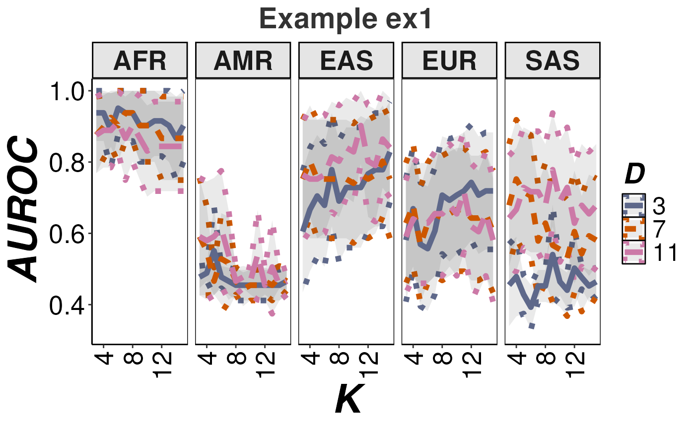
RAIDS performance for the synthtic data.
In this illustrative example, the performance estimates are lower than expected with a realistic sequence profile and a complete reference population file.
Format population reference dataset (optional)
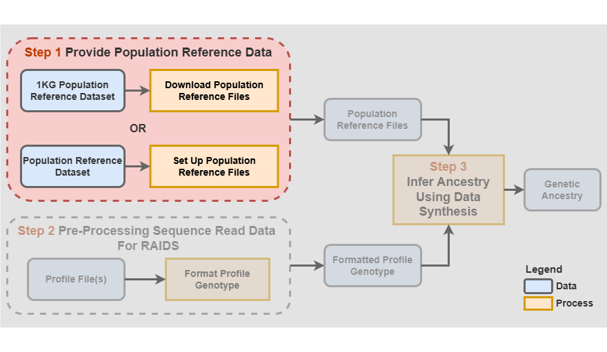
Step 1 - Provide population reference data
A population reference dataset with known ancestry is required to infer ancestry.
Three important reference files, containing formatted information about the reference dataset, are required:
- The population reference GDS File
- The population reference SNV Annotation GDS file
- The population reference SNV Retained VCF file (optional)
The formats of those files are described in the Population reference dataset GDS files vignette.
The reference files associated to the Cancer Research associated paper are available. Note that these pre-processed files are for 1000 Genomes (1KG), in hg38. The files are available here:
https://labshare.cshl.edu/shares/krasnitzlab/aicsPaper
The size of the 1KG GDS file is 15GB.
The 1KG GDS file is mapped on hg38 (Lowy-Gallego et al. 2019).
This section can be skipped if you choose to use the pre-processed files.
Session info
Here is the output of sessionInfo() in the environment
in which this document was compiled:
## R version 4.5.1 (2025-06-13)
## Platform: x86_64-pc-linux-gnu
## Running under: Ubuntu 24.04.3 LTS
##
## Matrix products: default
## BLAS:   /usr/lib/x86_64-linux-gnu/openblas-pthread/libblas.so.3
## LAPACK: /usr/lib/x86_64-linux-gnu/openblas-pthread/libopenblasp-r0.3.26.so;  LAPACK version 3.12.0
##
## locale:
##  [1] LC_CTYPE=en_US.UTF-8       LC_NUMERIC=C
##  [3] LC_TIME=en_US.UTF-8        LC_COLLATE=en_US.UTF-8
##  [5] LC_MONETARY=en_US.UTF-8    LC_MESSAGES=en_US.UTF-8
##  [7] LC_PAPER=en_US.UTF-8       LC_NAME=C
##  [9] LC_ADDRESS=C               LC_TELEPHONE=C
## [11] LC_MEASUREMENT=en_US.UTF-8 LC_IDENTIFICATION=C
##
## time zone: UTC
## tzcode source: system (glibc)
##
## attached base packages:
## [1] stats4    stats     graphics  grDevices utils     datasets  methods
## [8] base
##
## other attached packages:
##  [1] Matrix_1.7-3         RAIDS_1.7.3          Rsamtools_2.25.3
##  [4] Biostrings_2.77.2    XVector_0.49.1       GenomicRanges_1.61.5
##  [7] IRanges_2.43.5       S4Vectors_0.47.4     Seqinfo_0.99.2
## [10] BiocGenerics_0.55.1  generics_0.1.4       dplyr_1.1.4
## [13] GENESIS_2.39.3       SNPRelate_1.43.1     gdsfmt_1.45.1
## [16] knitr_1.50           BiocStyle_2.37.1
##
## loaded via a namespace (and not attached):
##   [1] RColorBrewer_1.1-3                jsonlite_2.0.0
##   [3] shape_1.4.6.1                     magrittr_2.0.4
##   [5] jomo_2.7-6                        GenomicFeatures_1.61.6
##   [7] farver_2.1.2                      logistf_1.26.1
##   [9] nloptr_2.2.1                      rmarkdown_2.30
##  [11] fs_1.6.6                          BiocIO_1.19.0
##  [13] ragg_1.5.0                        vctrs_0.6.5
##  [15] memoise_2.0.1                     minqa_1.2.8
##  [17] RCurl_1.98-1.17                   quantsmooth_1.75.0
##  [19] htmltools_0.5.8.1                 S4Arrays_1.9.1
##  [21] curl_7.0.0                        broom_1.0.10
##  [23] pROC_1.19.0.1                     SparseArray_1.9.1
##  [25] mitml_0.4-5                       sass_0.4.10
##  [27] bslib_0.9.0                       desc_1.4.3
##  [29] sandwich_3.1-1                    zoo_1.8-14
##  [31] cachem_1.1.0                      GenomicAlignments_1.45.4
##  [33] lifecycle_1.0.4                   iterators_1.0.14
##  [35] pkgconfig_2.0.3                   R6_2.6.1
##  [37] fastmap_1.2.0                     rbibutils_2.3
##  [39] MatrixGenerics_1.21.0             digest_0.6.37
##  [41] GWASTools_1.55.0                  AnnotationDbi_1.71.1
##  [43] textshaping_1.0.3                 RSQLite_2.4.3
##  [45] labeling_0.4.3                    httr_1.4.7
##  [47] abind_1.4-8                       mgcv_1.9-3
##  [49] compiler_4.5.1                    withr_3.0.2
##  [51] bit64_4.6.0-1                     S7_0.2.0
##  [53] backports_1.5.0                   BiocParallel_1.43.4
##  [55] DBI_1.2.3                         pan_1.9
##  [57] MASS_7.3-65                       quantreg_6.1
##  [59] DelayedArray_0.35.3               rjson_0.2.23
##  [61] DNAcopy_1.83.0                    tools_4.5.1
##  [63] lmtest_0.9-40                     nnet_7.3-20
##  [65] glue_1.8.0                        restfulr_0.0.16
##  [67] nlme_3.1-168                      grid_4.5.1
##  [69] gtable_0.3.6                      operator.tools_1.6.3
##  [71] BSgenome_1.77.2                   formula.tools_1.7.1
##  [73] class_7.3-23                      tidyr_1.3.1
##  [75] ensembldb_2.33.2                  data.table_1.17.8
##  [77] GWASExactHW_1.2                   stringr_1.5.2
##  [79] foreach_1.5.2                     pillar_1.11.1
##  [81] splines_4.5.1                     lattice_0.22-7
##  [83] survival_3.8-3                    rtracklayer_1.69.1
##  [85] bit_4.6.0                         SparseM_1.84-2
##  [87] BSgenome.Hsapiens.UCSC.hg38_1.4.5 tidyselect_1.2.1
##  [89] SeqVarTools_1.47.0                reformulas_0.4.1
##  [91] bookdown_0.45                     ProtGenerics_1.41.0
##  [93] SummarizedExperiment_1.39.2       RhpcBLASctl_0.23-42
##  [95] xfun_0.53                         Biobase_2.69.1
##  [97] matrixStats_1.5.0                 stringi_1.8.7
##  [99] UCSC.utils_1.5.0                  lazyeval_0.2.2
## [101] yaml_2.3.10                       boot_1.3-31
## [103] evaluate_1.0.5                    codetools_0.2-20
## [105] tibble_3.3.0                      BiocManager_1.30.26
## [107] cli_3.6.5                         rpart_4.1.24
## [109] systemfonts_1.3.1                 Rdpack_2.6.4
## [111] jquerylib_0.1.4                   Rcpp_1.1.0
## [113] GenomeInfoDb_1.45.12              png_0.1-8
## [115] XML_3.99-0.19                     parallel_4.5.1
## [117] MatrixModels_0.5-4                ggplot2_4.0.0
## [119] pkgdown_2.1.3                     blob_1.2.4
## [121] AnnotationFilter_1.33.0           bitops_1.0-9
## [123] lme4_1.1-37                       glmnet_4.1-10
## [125] SeqArray_1.49.8                   VariantAnnotation_1.55.1
## [127] scales_1.4.0                      purrr_1.1.0
## [129] crayon_1.5.3                      rlang_1.1.6
## [131] KEGGREST_1.49.1                   mice_3.18.0