Detection of consensus regions inside a group of experiments
Astrid Deschênes, Fabien Claude Lamaze, Pascal Belleau and Arnaud Droit
15 October, 2025
Source:vignettes/consensusSeekeR.Rmd
consensusSeekeR.RmdAbstract
This package compares genomic positions and genomic ranges from multiple experiments to extract common regions. The size of the analyzed region is adjustable as well as the number of experiences in which a feature must be present in a potential region to tag this region as a consensus region. In genomic analysis where feature identification generates a position value surrounded by a genomic range, such as ChIP-Seq peaks and nucleosome positions, the replication of an experiment may result in slight differences between predicted values. This package enables the conciliation of the results into consensus regions.Licensing and citing
This package and the underlying consensusSeekeR code are distributed under the Artistic license 2.0. You are free to use and redistribute this software.
If you use this package for a publication, we would ask you to cite the following:
Samb R, Khadraoui K, Belleau P, et al. (2015) Using informative Multinomial-Dirichlet prior in a t-mixture with reversible jump estimation of nucleosome positions for genome-wide profiling. Statistical Applications in Genetics and Molecular Biology. Published online before print December 10, 2015. doi:10.1515/sagmb-2014-0098
Introduction
Genome data, such as genes, nucleosomes or single-nucleotide polymorphisms (SNPs) are linked to the genome by occupying either a range of positions or a single position on the sequence. Genomic related data integration is made possible by treating the data as ranges on the genome (Lawrence et al. 2013). Bioconductor has developed an infrastructure, including packages such as GenomicRanges, IRanges and GenomicFeatures, which facilitate the integrative statistical analysis of range-based genomic data.
Ranges format is a convenient way for the analysis of diffent experimental genomic data. As an example, the peak calling step, in the analysis of ChIP-seq data, commonly generates NarrowPeak outputs. The NarrowPeak format, wich is used by the ENCODE project (Dunham et al. 2012), includes a peak position located inside a genomic range.
In genomic analysis where feature identification generate a position value surrounded by a genomic range, such as ChIP-Seq peaks and nucleosome postions, the replication of an experiment may result in slight differences between predicted values. Conciliation of the results can be difficult, especially when many replicates are done. One current approach used to identify consensus regions in a group of results consist of extracting the overlapping regions of the genomic ranges. This approach, when used on a large number of experiments, can miss, as a side effect, regions when one of the experiment has missing or slightly shift features. On the other hand, the use of the union of the regions can result in wide consensus ranges.
As an example, the Figure @ref(fig:peakRegion) shows, using Integrative genomics viewer (Robinson et al. 2011), two ChIP-Seq peaks from ENCODE for the FOSL2 transcription factor (DCC accession: ENCFF002CFN). The data have been analyzed using MACS2 (Zhang et al. 2008) with the default parameters and the q-value set to 0.05. The ChIP-Seq peak is a genomic feature that can be defined by a position value (the peak position) and a genome range (the enriched region). This example shows that the peak position is not necessarily at the center of the enriched region.
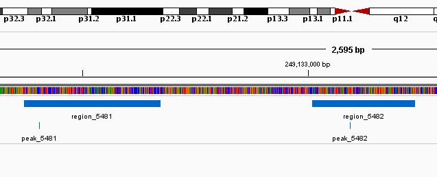
The consensusSeekeR package implements a novative way to identify consensus which use the features positions, instead of the most commonly used genomic ranges.
The consensusSeekeR package
The consensusSeekeR package implements a novative way to identify consensus ranges in a group of experiments which generated position values surrounded by genomic ranges. The consensusSeekeR package is characterized by its use of the position values, instead of the genomic ranges, to identify the consensus regions. The positions values have the double advantages of being, most of the time, the most important information from features and allowing creation of consensius regions of smaller ranges.
Using iterative steps on ordered features position values from all experiments, a window of fixed size (specified by user) with the current feature position as starting point is set. All features which reside inside the window are gathered to calculate a median feature position which is then used to recreate a new window. This time, the new window has twice the size fixed by user and its center is the median feature position. An update of the features located inside the window is done and the median feature position is recalculated. This step is repeated up to the moment that the set of features remains identical between two iterations. The final set of features positions is used to fix the central position of the consensus region. This final region must respect the minimum number of experiments with at least one feature inside it to be retained as a final consensus region. The minimum number of experiments is set by the user. At last, the consensus region can be extended or/and shrinked to fit the regions associated to the position values present inside. If new features positions are added during the consensus region resizing, the iterative steps are not reprocessed. It is possible that the extension step adds new features in the extended consensus region. However, those new features ranges won’t be taken into account during the extension step.
Loading consensusSeekeR package
As with any R package, the consensusSeekeR package should first be loaded with the following command:
Inputs
Positions and Ranges
The main function of the consensusSeekeR
is findConsensusPeakRegions. The mains inputs of the
findConsensusPeakRegions function are:
- a
GRangesof the featurepositionsof all experiments with a metadata field calledname. - a
GRangesof the featurerangesfor all experiments with a metadata field calledname.
Beware that the GRanges of the feature
ranges is only mandatory if the
expandToFitPeakRegion parameter and/or the
shrinkToFitPeakRegion parameter are set to
TRUE.
Both inputs must satify these conditions:
- All rows of each
GRangesmust be named after the experiment source. All entries from the same experiment must be assigned the same name. - Each feature must have one entry in both
GRanges. The metadata fieldnameis used to associate the feature position to its range.
This is an example showing how a metadata field name can
easily be created and row names can be assigned:
### Initial dataset without metadata field
head(A549_FOSL2_01_NarrowPeaks_partial, n = 3)
## GRanges object with 3 ranges and 0 metadata columns:
##       seqnames              ranges strand
##          <Rle>           <IRanges>  <Rle>
##   [1]     chr1 249119914-249120249      *
##   [2]     chr1 249120596-249121174      *
##   [3]     chr1 249123089-249123453      *
##   -------
##   seqinfo: 25 sequences from an unspecified genome; no seqlengths

### Adding a new metadata field "name" unique to each entry
A549_FOSL2_01_NarrowPeaks_partial$name <- paste0("FOSL2_01_entry_",
                                1:length(A549_FOSL2_01_NarrowPeaks_partial))

### Assign the same row name to each entry
names(A549_FOSL2_01_NarrowPeaks_partial) <- rep("FOSL2_01",
                                length(A549_FOSL2_01_NarrowPeaks_partial))

### Final dataset with metadata field 'name' and row names
head(A549_FOSL2_01_NarrowPeaks_partial, n = 3)
## GRanges object with 3 ranges and 1 metadata column:
##            seqnames              ranges strand |             name
##               <Rle>           <IRanges>  <Rle> |      <character>
##   FOSL2_01     chr1 249119914-249120249      * | FOSL2_01_entry_1
##   FOSL2_01     chr1 249120596-249121174      * | FOSL2_01_entry_2
##   FOSL2_01     chr1 249123089-249123453      * | FOSL2_01_entry_3
##   -------
##   seqinfo: 25 sequences from an unspecified genome; no seqlengths
Chromosomes information
The chromosomes information is mandatory. It ensures that the consensus regions do not exceed the length of the chromosomes.
The chromosomes information is contained inside a
Seqinfo object. The information from some UCSC genomes can
be fetched automatically using the Seqinfo
package.
### Import library
library(Seqinfo)

### Get the information for Human genome version 19
hg19Info <- Seqinfo(genome="hg19")

### Subset the object to keep only the analyzed chromosomes
hg19Subset <- hg19Info[c("chr1", "chr10", "chrX")]
A Seqinfo object can also be created using the
chromosomes information specific to the analyzed genome.
Read NarrowPeak files
The NarrowPeak format is often used to provide called peaks of signal enrichment based on pooled, normalized data. The rtracklayer package has functions which faciliates the loading of NarrowPeak files.
Since the main function of the consensusSeekeR
package needs 2 GRanges objects, some manipulations are
needed to create one GRanges for the regions and one
GRanges for the peaks.
### Load the needed packages
library(rtracklayer)
library(GenomicRanges)

### Demo file contained within the consensusSeekeR package
file_narrowPeak <- system.file("extdata",
        "A549_FOSL2_ENCSR000BQO_MZW_part_chr_1_and_12.narrowPeak", package = "consensusSeekeR")

### Information about the extra columns present in the file need
### to be specified
extraCols <- c(signalValue = "numeric", pValue = "numeric", qValue = "numeric", peak = "integer")

### Create genomic ranges for the regions
regions <- import(file_narrowPeak, format = "BED", extraCols = extraCols)

### Create genomic ranges for the peaks
peaks           <-  regions
ranges(peaks)   <-  IRanges(start = (start(regions) + regions$peak), width = rep(1, length(regions$peak)))

### First rows of each GRanges object
head(regions, n = 2)
## GRanges object with 2 ranges and 6 metadata columns:
##       seqnames        ranges strand |                   name     score
##          <Rle>     <IRanges>  <Rle> |            <character> <numeric>
##   [1]     chr1 846589-846847      * | peaks/Hosa_A549_FOSL..        57
##   [2]     chr1 856004-856159      * | peaks/Hosa_A549_FOSL..        43
##       signalValue    pValue    qValue      peak
##         <numeric> <numeric> <numeric> <integer>
##   [1]     5.59984   8.75159   5.77648        98
##   [2]     5.16770   7.21902   4.33609       108
##   -------
##   seqinfo: 2 sequences from an unspecified genome; no seqlengths
head(peaks, n = 2)
## GRanges object with 2 ranges and 6 metadata columns:
##       seqnames    ranges strand |                   name     score signalValue
##          <Rle> <IRanges>  <Rle> |            <character> <numeric>   <numeric>
##   [1]     chr1    846687      * | peaks/Hosa_A549_FOSL..        57     5.59984
##   [2]     chr1    856112      * | peaks/Hosa_A549_FOSL..        43     5.16770
##          pValue    qValue      peak
##       <numeric> <numeric> <integer>
##   [1]   8.75159   5.77648        98
##   [2]   7.21902   4.33609       108
##   -------
##   seqinfo: 2 sequences from an unspecified genome; no seqlengths
A simpler way is to use the readNarrowPeakFile function
of the consensusSeekeR
package which generates both the peaks and the narrowPeak
GRanges.
library(consensusSeekeR)

### Demo file contained within the consensusSeekeR package
file_narrowPeak <- system.file("extdata",
    "A549_FOSL2_ENCSR000BQO_MZW_part_chr_1_and_12.narrowPeak", package = "consensusSeekeR")

### Create genomic ranges for both the regions and the peaks
result <- readNarrowPeakFile(file_narrowPeak, extractRegions = TRUE, extractPeaks = TRUE)

### First rows of each GRanges object
head(result$narrowPeak, n = 2)
## GRanges object with 2 ranges and 6 metadata columns:
##       seqnames        ranges strand |                   name     score
##          <Rle>     <IRanges>  <Rle> |            <character> <numeric>
##   [1]     chr1 846589-846847      * | peaks/Hosa_A549_FOSL..        57
##   [2]     chr1 856004-856159      * | peaks/Hosa_A549_FOSL..        43
##       signalValue    pValue    qValue      peak
##         <numeric> <numeric> <numeric> <integer>
##   [1]     5.59984   8.75159   5.77648        98
##   [2]     5.16770   7.21902   4.33609       108
##   -------
##   seqinfo: 2 sequences from an unspecified genome; no seqlengths
head(result$peak, n = 2)
## GRanges object with 2 ranges and 6 metadata columns:
##       seqnames    ranges strand |                   name     score signalValue
##          <Rle> <IRanges>  <Rle> |            <character> <numeric>   <numeric>
##   [1]     chr1    846687      * | peaks/Hosa_A549_FOSL..        57     5.59984
##   [2]     chr1    856112      * | peaks/Hosa_A549_FOSL..        43     5.16770
##          pValue    qValue      peak
##       <numeric> <numeric> <integer>
##   [1]   8.75159   5.77648        98
##   [2]   7.21902   4.33609       108
##   -------
##   seqinfo: 2 sequences from an unspecified genome; no seqlengths
Case study: nucleosome positioning
Global gene expression patterns are established and maintained by the concerted actions of Transcription Factors (TFs) and the proteins that constitute chromatin. The key structural element of chromatin is the nucleosome, which consists of an octameric histone core wrapped by 147 bps of DNA and connected to its neighbor by approximately 10-80 pbs of linker DNA (Kornberg and Lorch 1999). Nucleosome occupancy and positioning have been proved to be dynamic. It also has a major impact on expression, regulation, and evolution of eukaryotic genes (Jiang et al. 2015).
Comparing nucleosome positioning results from different software
With the development of Next-generation sequencing, nucleosome positioning using MNase-Seq data or MNase- or sonicated- ChIP-Seq data combined with either single-end or paired-end sequencing have evolved as popular techniques. Software such as PING (Woo et al. 2013) and NOrMAL (Polishko et al. 2012), generates output which contains the positions of the predicted nucleosomes, which simply are one base pair positions on the reference genome. This position represents the center of the predicted nucleosome. A range of 73 bps is usually superposed to the predicted nucleosome to repesent the nucleosome occupancy.
First, the consensusSeekeR package must be loaded.
The datasets, which are included in the consensusSeekeR package, have to be loaded. Those include results obtained using syntethic reads distributed following a normal distribution with a variance of 20 from three different nucleosome positioning software: PING (Woo et al. 2013), NOrMAL (Polishko et al. 2012) and NucPosSimulator (Schöpflin et al. 2013). The genomic ranges have been obtained by adding 73 bps to the detected positions.
### Loading dataset from NOrMAL
data(NOrMAL_nucleosome_positions) ; data(NOrMAL_nucleosome_ranges)

### Loading dataset from PING
data(PING_nucleosome_positions) ; data(PING_nucleosome_ranges)

### Loading dataset from NucPosSimulator
data(NucPosSimulator_nucleosome_positions) ; data(NucPosSimulator_nucleosome_ranges)
For the positions and ranges dataset from the same software, the
name field is paired to ensure that each position can be
associated to its range. The metadata field name must be
unique to each feature for all datasets.
### Each entry in the positions dataset has an equivalent metadata
### "name" entry in the ranges dataset
head(NOrMAL_nucleosome_positions, n = 2)
## GRanges object with 2 ranges and 1 metadata column:
##          seqnames    ranges strand |     name
##             <Rle> <IRanges>  <Rle> | <factor>
##   NOrMAL     chr1     10240      + |      no1
##   NOrMAL     chr1     10409      + |      no2
##   -------
##   seqinfo: 1 sequence from an unspecified genome; no seqlengths

head(NOrMAL_nucleosome_ranges, n = 2)
## GRanges object with 2 ranges and 1 metadata column:
##          seqnames      ranges strand |     name
##             <Rle>   <IRanges>  <Rle> | <factor>
##   NOrMAL     chr1 10167-10313      + |      no1
##   NOrMAL     chr1 10336-10482      + |      no2
##   -------
##   seqinfo: 1 sequence from an unspecified genome; no seqlengths
To be able to identify all entries from the same software, each row of the dataset has to be assigned a name. All positions and ranges from the same source must be assigned identical row names. In this exemple, datasets are going to be identified by the name of their source software.
### Assigning software name "NOrMAL"
names(NOrMAL_nucleosome_positions) <- rep("NOrMAL", length(NOrMAL_nucleosome_positions))
names(NOrMAL_nucleosome_ranges) <- rep("NOrMAL", length(NOrMAL_nucleosome_ranges))

### Assigning experiment name "PING"
names(PING_nucleosome_positions) <- rep("PING", length(PING_nucleosome_positions))
names(PING_nucleosome_ranges) <- rep("PING", length(PING_nucleosome_ranges))

### Assigning experiment name "NucPosSimulator"
names(NucPosSimulator_nucleosome_positions) <- rep("NucPosSimulator",
                                length(NucPosSimulator_nucleosome_positions))
names(NucPosSimulator_nucleosome_ranges) <- rep("NucPosSimulator",
                                length(NucPosSimulator_nucleosome_ranges))

### Row names are unique to each software
head(NOrMAL_nucleosome_positions, n = 2)
## GRanges object with 2 ranges and 1 metadata column:
##          seqnames    ranges strand |     name
##             <Rle> <IRanges>  <Rle> | <factor>
##   NOrMAL     chr1     10240      + |      no1
##   NOrMAL     chr1     10409      + |      no2
##   -------
##   seqinfo: 1 sequence from an unspecified genome; no seqlengths

head(PING_nucleosome_positions, n = 2)
## GRanges object with 2 ranges and 1 metadata column:
##        seqnames    ranges strand |     name
##           <Rle> <IRanges>  <Rle> | <factor>
##   PING     chr1     10075      + |       p1
##   PING     chr1     10241      + |       p2
##   -------
##   seqinfo: 1 sequence from an unspecified genome; no seqlengths

head(NucPosSimulator_nucleosome_positions, n = 2)
## GRanges object with 2 ranges and 1 metadata column:
##                   seqnames    ranges strand |     name
##                      <Rle> <IRanges>  <Rle> | <factor>
##   NucPosSimulator     chr1     10075      + |      nu1
##   NucPosSimulator     chr1     10241      + |      nu2
##   -------
##   seqinfo: 1 sequence from an unspecified genome; no seqlengths
The consensus regions for chromosome 1 only are calculated with a
defaut region size of 50 bases pairs (2 * extendingSize)
The regions are extended to include all nucleosome regions
(expandToFitPeakRegion = TRUE and
shrinkToFitPeakRegion = TRUE). To be retained
as a consensus region, nucleosomes from at least 2 software must be
present in the region (minNbrExp = 2). .
### Only choromsome 1 is going to be analyzed
chrList <- Seqinfo("chr1", 135534747, NA)

### Find consensus regions with both replicates inside it
results <- findConsensusPeakRegions(
            narrowPeaks = c(NOrMAL_nucleosome_ranges, PING_nucleosome_ranges,
                                NucPosSimulator_nucleosome_ranges),
            peaks = c(NOrMAL_nucleosome_positions, PING_nucleosome_positions,
                                NucPosSimulator_nucleosome_positions),
            chrInfo = chrList,
            extendingSize = 25,
            expandToFitPeakRegion = TRUE,
            shrinkToFitPeakRegion = TRUE,
            minNbrExp = 2,
            nbrThreads = 1)
The output of findConsensusPeakRegions function is a
list containing an object call and an object
consensusRanges. The object call contains the
matched call while the object consensusRanges is a
GRanges containing the consensus regions.
### Print the call
results$call
## findConsensusPeakRegions(narrowPeaks = c(NOrMAL_nucleosome_ranges,
##     PING_nucleosome_ranges, NucPosSimulator_nucleosome_ranges),
##     peaks = c(NOrMAL_nucleosome_positions, PING_nucleosome_positions,
##         NucPosSimulator_nucleosome_positions), chrInfo = chrList,
##     extendingSize = 25, expandToFitPeakRegion = TRUE, shrinkToFitPeakRegion = TRUE,
##     minNbrExp = 2, nbrThreads = 1)

### Print the 3 first consensus regions
head(results$consensusRanges, n = 3)
## GRanges object with 3 ranges and 0 metadata columns:
##       seqnames      ranges strand
##          <Rle>   <IRanges>  <Rle>
##   [1]     chr1 10002-10148      *
##   [2]     chr1 10167-10314      *
##   [3]     chr1 10334-10482      *
##   -------
##   seqinfo: 1 sequence from an unspecified genome; no seqlengths
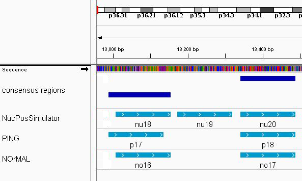
A total of 27 consensus regions have been found. An exemple of the consensus regions (in dark blue) is shown in Figure @ref(fig:nucleosomes) using Integrative genomics viewer (Robinson et al. 2011):
Case study: ChIP-Seq data
Next-generation DNA sequencing coupled with chromatin immunoprecipitation (ChIP-seq) has changed the ability to interrogate the genomic landscape of histone modifications, transcriptional cofactors and transcription-factors binding in living cells (Mundade et al. 2014). Consortium, such as ENCODE have developed and are constantly updating a set of standards and guidelines for ChIP-Seq experiments (Landt and Marinov 2012).
ChIP-seq combines chromatin immunoprecipitation (ChIP) with massively parallel DNA sequencing. The obtained sequence reads are first mapped to the reference genome of the organism used in the experiments. Binding sites are then detected using software specialized in transcript factor binding sites identification, such as MACS2 (Zhang et al. 2008) and PeakRanger (Feng et al. 2011). Peaks are defined as a single base pair position while statistically enriched regions are defined as genomic ranges.
ChIP-Seq replicates from one experiment
The Encyclopedia of DNA Elements (ENCODE) Consortium is an international collaboration of research groups funded by the National Human Genome Research Institute. The ENCODE website is a portal giving access to the data generated by the ENCODE Consortium. The amount of data gathered is extensive. Moreover, for some experiments, more than one ChIP-Seq replicate is often available.
The software used to identify transcript factor binding sites generally generates a peak position and an enriched region for each binding site. However, it is quite unlikely that the exact peak position is exactly the same across replicates. Even more, there is not yet a consensus on how to analyze multiple-replicate ChIP-seq samples (Yang et al. 2014).
The consensusSeekeR package can be used to identify consensus regions for two or more replicates ChIP-Seq samples. The consensus regions are being found by using the peak positions.
The transcription factor binding for the CTCF transcription factor have been analyzed and 2 replicates are available in BAM files format on ENCODE website (DCCs: ENCFF000MYJ and ENCFF000MYN). The NarrowPeaks were generated using MACS2 (Zhang et al. 2008) with the default parameters and the q-value set to 0.05.
To simplify this demo, only part of genome hg19, chr1:246000000-249250621 and chr10:10000000-12500000, have been retained in the datasets.
First, the consensusSeekeR package must be loaded.
The datasets, which are included in the consensusSeekeR package, have to be loaded.
### Loading datasets
data(A549_CTCF_MYN_NarrowPeaks_partial) ; data(A549_CTCF_MYN_Peaks_partial)
data(A549_CTCF_MYJ_NarrowPeaks_partial) ; data(A549_CTCF_MYJ_Peaks_partial)
To be able to identify data from the same source, each row of the
dataset has to be assigned a source name. Beware that
NarrowPeak and Peak datasets from the same
source must be assigned identical names. In this exemple, datasets are
replicates of the same experiment. So, the names “rep01” and “rep02” are
going to be assigned to each dataset.
### Assigning experiment name "rep01" to the first replicate
names(A549_CTCF_MYJ_NarrowPeaks_partial) <- rep("rep01", length(A549_CTCF_MYJ_NarrowPeaks_partial))
names(A549_CTCF_MYJ_Peaks_partial)       <- rep("rep01", length(A549_CTCF_MYJ_Peaks_partial))

### Assigning experiment name "rep02" to the second replicate
names(A549_CTCF_MYN_NarrowPeaks_partial) <- rep("rep02", length(A549_CTCF_MYN_NarrowPeaks_partial))
names(A549_CTCF_MYN_Peaks_partial)       <- rep("rep02", length(A549_CTCF_MYN_Peaks_partial))
The consensus regions for chromosome 10 only are calculated with a
defaut region size of 200 bases pairs (2 * extendingSize)
The regions are extended to include all peaks regions
(expandToFitPeakRegion = TRUE and
shrinkToFitPeakRegion = TRUE). A peak from
both replicates must be present withinin a region for it to be retained
as a consensus region.
### Only choromsome 10 is going to be analyzed
chrList <- Seqinfo("chr10", 135534747, NA)

### Find consensus regions with both replicates inside it
results <- findConsensusPeakRegions(
            narrowPeaks = c(A549_CTCF_MYJ_NarrowPeaks_partial, A549_CTCF_MYN_NarrowPeaks_partial),
            peaks = c(A549_CTCF_MYJ_Peaks_partial, A549_CTCF_MYN_Peaks_partial),
            chrInfo = chrList,
            extendingSize = 100,
            expandToFitPeakRegion = TRUE,
            shrinkToFitPeakRegion = TRUE,
            minNbrExp = 2,
            nbrThreads = 1)
The output of findConsensusPeakRegions function is a
list containing an object call and an object
conesensusRanges. The object call contains the
matched call while the object conesensusRanges is a
GRanges containing the consensus regions.
### Print the call
results$call
## findConsensusPeakRegions(narrowPeaks = c(A549_CTCF_MYJ_NarrowPeaks_partial,
##     A549_CTCF_MYN_NarrowPeaks_partial), peaks = c(A549_CTCF_MYJ_Peaks_partial,
##     A549_CTCF_MYN_Peaks_partial), chrInfo = chrList, extendingSize = 100,
##     expandToFitPeakRegion = TRUE, shrinkToFitPeakRegion = TRUE,
##     minNbrExp = 2, nbrThreads = 1)

### Print the 3 first consensus regions
head(results$consensusRanges, n = 3)
## GRanges object with 3 ranges and 0 metadata columns:
##       seqnames            ranges strand
##          <Rle>         <IRanges>  <Rle>
##   [1]    chr10 11078504-11078657      *
##   [2]    chr10 11312608-11312835      *
##   [3]    chr10 11466554-11466858      *
##   -------
##   seqinfo: 1 sequence from an unspecified genome; no seqlengths
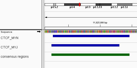
A total of 18 consensus regions have been found. An example of the consensus regions (in green) is shown in Figure @ref(fig:ctcf), using Integrative genomics viewer (Robinson et al. 2011).
ChIP-Seq data from multiple experiments
The consensusSeekeR package can also be used to identify consensus regions for two or more ChIP-Seq samples from multiple experiments. The peak positions are the feature used to identify the consensus regions.
The transcription factor binding for the NR3C1 transcription factor have been analyzed in more than one experiment. For each experiment, replicates have been analyzed together using the irreproducible discovery rate method (Li et al. 2011). Results are available in bed narrowPeak format on ENCODE website (DCCs: ENCFF002CFQ, ENCFF002CFR and ENCFF002CFS) (Dunham et al. 2012).
To simplify this demo, only part of genome hg19, chr2:40000000-50000000 and chr3:10000000-13000000, have been retained in the datasets.
First, the consensusSeekeR package must be loaded.
The datasets, which are included in the consensusSeekeR package, have to be loaded.
### Loading datasets
data(A549_NR3C1_CFQ_NarrowPeaks_partial) ; data(A549_NR3C1_CFQ_Peaks_partial)
data(A549_NR3C1_CFR_NarrowPeaks_partial) ; data(A549_NR3C1_CFR_Peaks_partial)
data(A549_NR3C1_CFS_NarrowPeaks_partial) ; data(A549_NR3C1_CFS_Peaks_partial)
To be able to identify data from the same source, each row of the dataset has to be assigned an experiment name. Beware that NarrowPeak and Peak datasets from the same source must be assigned identical names. In this exemple, datasets are coming from different experiments for the same transcription factor. So, the short name of each experiment “ENCFF002CFQ”, “ENCFF002CFR” and “ENCFF002CFS” is going to be assigned to each dataset.
### Assign experiment name "ENCFF002CFQ" to the first experiment
names(A549_NR3C1_CFQ_NarrowPeaks_partial) <- rep("ENCFF002CFQ",
                                length(A549_NR3C1_CFQ_NarrowPeaks_partial))
names(A549_NR3C1_CFQ_Peaks_partial) <- rep("ENCFF002CFQ",
                                length(A549_NR3C1_CFQ_Peaks_partial))

### Assign experiment name "ENCFF002CFQ" to the second experiment
names(A549_NR3C1_CFR_NarrowPeaks_partial) <- rep("ENCFF002CFR",
                                length(A549_NR3C1_CFR_NarrowPeaks_partial))
names(A549_NR3C1_CFR_Peaks_partial)       <- rep("ENCFF002CFR",
                                length(A549_NR3C1_CFR_Peaks_partial))

### Assign experiment name "ENCFF002CFQ" to the third experiment
names(A549_NR3C1_CFS_NarrowPeaks_partial) <- rep("ENCFF002CFS",
                                length(A549_NR3C1_CFS_NarrowPeaks_partial))
names(A549_NR3C1_CFS_Peaks_partial)       <- rep("ENCFF002CFS",
                                length(A549_NR3C1_CFS_Peaks_partial))
In ENCODE bed narrowPeak format, entries don’t have a specific
metadata field called name. So, to be able to use the
findConsensusPeakRegions function, specific names must
manually be added to each entry.
### Assign specific name to each entry of to first experiment
### NarrowPeak name must fit Peaks name for same experiment
A549_NR3C1_CFQ_NarrowPeaks_partial$name <- paste0("NR3C1_CFQ_region_",
                                1:length(A549_NR3C1_CFQ_NarrowPeaks_partial))
A549_NR3C1_CFQ_Peaks_partial$name       <- paste0("NR3C1_CFQ_region_",
                                1:length(A549_NR3C1_CFQ_NarrowPeaks_partial))

### Assign specific name to each entry of to second experiment
### NarrowPeak name must fit Peaks name for same experiment
A549_NR3C1_CFR_NarrowPeaks_partial$name <- paste0("NR3C1_CFR_region_",
                                1:length(A549_NR3C1_CFR_NarrowPeaks_partial))
A549_NR3C1_CFR_Peaks_partial$name       <- paste0("NR3C1_CFR_region_",
                                1:length(A549_NR3C1_CFR_Peaks_partial))

### Assign specific name to each entry of to third experiment
### NarrowPeak name must fit Peaks name for same experiment
A549_NR3C1_CFS_NarrowPeaks_partial$name <- paste0("NR3C1_CFS_region_",
                                1:length(A549_NR3C1_CFS_NarrowPeaks_partial))
A549_NR3C1_CFS_Peaks_partial$name       <- paste0("NR3C1_CFS_region_",
                                1:length(A549_NR3C1_CFS_Peaks_partial))
The consensus regions for chromosome 2 only are calculated with a
defaut region size of 400 bases pairs (2 * extendingSize)
The regions are not extended to include all peaks regions but are
shrinked when exceeding peaks regions
(expandToFitPeakRegion = FALSE and
shrinkToFitPeakRegion = TRUE). A peak from 2
out of 3 experiments must be present in a region for it to be retained
as a consensus region.
### Only choromsome 2 is going to be analyzed
chrList <- Seqinfo("chr2", 243199373, NA)

### Find consensus regions with both replicates inside it
results <- findConsensusPeakRegions(
            narrowPeaks = c(A549_NR3C1_CFQ_NarrowPeaks_partial,
                        A549_NR3C1_CFR_NarrowPeaks_partial,
                        A549_NR3C1_CFS_NarrowPeaks_partial),
            peaks = c(A549_NR3C1_CFQ_Peaks_partial,
                        A549_NR3C1_CFR_Peaks_partial,
                        A549_NR3C1_CFS_Peaks_partial),
            chrInfo = chrList,
            extendingSize = 200,
            expandToFitPeakRegion = FALSE,
            shrinkToFitPeakRegion = TRUE,
            minNbrExp = 2,
            nbrThreads = 1)
The output of findConsensusPeakRegions function is a
list containing an object call and an object
consensusRanges. The object call contains the
matched call while the object consensusRanges is a
GRanges containing the consensus regions.
### Print the call
results$call
## findConsensusPeakRegions(narrowPeaks = c(A549_NR3C1_CFQ_NarrowPeaks_partial,
##     A549_NR3C1_CFR_NarrowPeaks_partial, A549_NR3C1_CFS_NarrowPeaks_partial),
##     peaks = c(A549_NR3C1_CFQ_Peaks_partial, A549_NR3C1_CFR_Peaks_partial,
##         A549_NR3C1_CFS_Peaks_partial), chrInfo = chrList, extendingSize = 200,
##     expandToFitPeakRegion = FALSE, shrinkToFitPeakRegion = TRUE,
##     minNbrExp = 2, nbrThreads = 1)

### Print the first 3 consensus regions
head(results$consensusRanges, n = 3)
## GRanges object with 3 ranges and 0 metadata columns:
##       seqnames            ranges strand
##          <Rle>         <IRanges>  <Rle>
##   [1]     chr2 42054830-42055168      *
##   [2]     chr2 42075261-42075544      *
##   [3]     chr2 42153872-42154111      *
##   -------
##   seqinfo: 1 sequence from an unspecified genome; no seqlengths
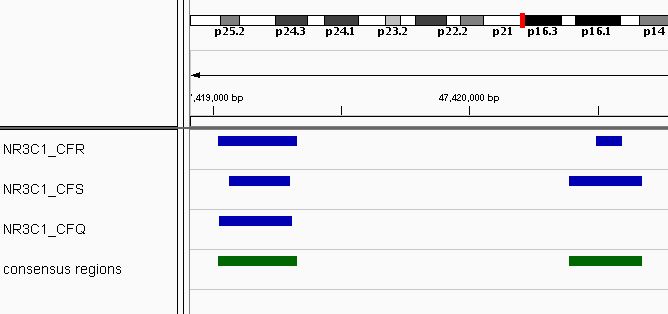
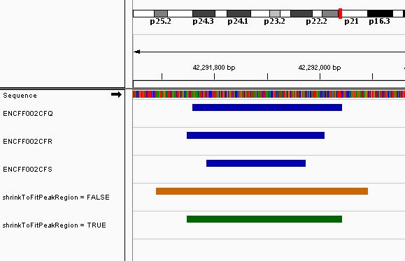
A total of 99 consensus regions have been found. A example of the consensus regions (in green) is shown in Figure @ref(fig:NR3C1) using Integrative genomics viewer (Robinson et al. 2011).
Parameters
Effect of the shrinkToFitPeakRegion parameter
The shrinkToFitPeakRegion allows the resizing of the
consensus region to fit the minimum regions of the included features
when those values are included inside the initial consensus region. When
the extendingSize parameter is large, the effect can be
quite visible on the final consensus regions. For exemple, Figure
@ref(fig:shrink) shows the same region, from the NR3C1 example with
extendingSize of 200, when the
shrinkToFitPeakRegion is set to TRUE (green
color) and to FALSE (orange color) using Integrative
genomics viewer (Robinson et al.
2011).
Effect of the expandToFitPeakRegion parameter
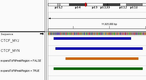
The expandToFitPeakRegion allows the resizing of the
consensus region to fit the maximum of the included features when those
values are outside the initial consensus region. When the
extendingSize parameter is small, the effect can be quite
visible on the final consensus regions. For exemple, the following
figure shows the same region, from the CTCF example with
extendingSize of 100, when the
shrinkToFitPeakRegion is set to FALSE (orange
color) and to TRUE (green color).
Effect of the extendingSize parameter
The value of the extendingSize parameter can affect the
final number of consensus regions. While small
extendingSize value can miss some regions, large
extendingSize value can gather consensus regions. Testing a
range of extendingSize parameters can be an option worth
considering.
As an example, the number of consensus regions obtained with
different values of extendingSize is calculated.
### Set different values for the extendingSize parameter
size <- c(1, 10, 50, 100, 300, 500, 750, 1000)

### Only chrompsome 10 is going to be analyzed
chrList <- Seqinfo("chr10", 135534747, NA)

### Find consensus regions using all the size values
resultsBySize <- lapply(size, FUN = function(size) findConsensusPeakRegions(
                    narrowPeaks = c(A549_CTCF_MYJ_NarrowPeaks_partial,
                                    A549_CTCF_MYN_NarrowPeaks_partial),
                    peaks = c(A549_CTCF_MYJ_Peaks_partial,
                                    A549_CTCF_MYN_Peaks_partial),
                    chrInfo = chrList,
                    extendingSize = size,
                    expandToFitPeakRegion = TRUE,
                    shrinkToFitPeakRegion = TRUE,
                    minNbrExp = 2,
                    nbrThreads = 1))

### Extract the number of consensus regions obtained for each extendingSize
nbrRegions <- mapply(resultsBySize,
                FUN = function(x) return(length(x$consensusRanges)))
A graph can be used to visualize the variation of the number of
consensus regions in function of the extendingSize
parameter (see Figure @ref(fig:sizeEffectG)).
library(ggplot2)

data <- data.frame(extendingSize = size, nbrRegions = nbrRegions)

ggplot(data, aes(extendingSize, nbrRegions)) + scale_x_log10("Extending size") +
        stat_smooth(se = FALSE, method = "loess", size=1.4) +
        ylab("Number of consensus regions") +
        ggtitle(paste0("Number of consensus regions in function of the extendingSize"))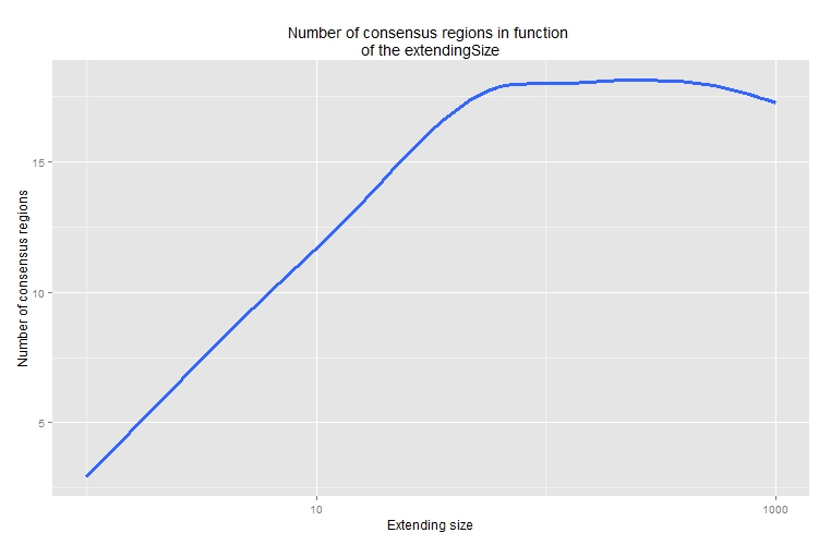
Parallelizing consensusSeekeR
Due to the size of the analyzed genomes, the
findConsensusPeakRegions function can take a while to
process. However, a job can be separated by chromosome and run in
parallel. This takes advantage of multiple processors and reduce the
total execution time. The number of threads used can be set with the
nbrThreads parameter in the
findConsensusPeakRegions function.
### Load data
data(A549_FOSL2_01_NarrowPeaks_partial) ; data(A549_FOSL2_01_Peaks_partial)
data(A549_FOXA1_01_NarrowPeaks_partial) ; data(A549_FOXA1_01_Peaks_partial)

### Assigning name "FOSL2"
names(A549_FOSL2_01_NarrowPeaks_partial) <- rep("FOSL2",
                                    length(A549_FOSL2_01_NarrowPeaks_partial))
names(A549_FOSL2_01_Peaks_partial)       <- rep("FOSL2",
                                    length(A549_FOSL2_01_Peaks_partial))

### Assigning name "FOXA1"
names(A549_FOXA1_01_NarrowPeaks_partial) <- rep("FOXA1",
                                    length(A549_FOXA1_01_NarrowPeaks_partial))
names(A549_FOXA1_01_Peaks_partial)       <- rep("FOXA1",
                                    length(A549_FOXA1_01_Peaks_partial))

### Two chromosomes to analyse
chrList <- Seqinfo(paste0("chr", c(1,10)), c(249250621, 135534747), NA)

### Find consensus regions using 2 threads
results <- findConsensusPeakRegions(
            narrowPeaks = c(A549_FOSL2_01_NarrowPeaks_partial,
                            A549_FOXA1_01_Peaks_partial),
            peaks = c(A549_FOSL2_01_Peaks_partial,
                            A549_FOXA1_01_NarrowPeaks_partial),
            chrInfo = chrList, extendingSize = 200, minNbrExp = 2,
            expandToFitPeakRegion = FALSE, shrinkToFitPeakRegion = FALSE,
nbrThreads = 4)Session info
Here is the output of sessionInfo() on the system on
which this document was compiled:
## R version 4.5.1 (2025-06-13)
## Platform: x86_64-pc-linux-gnu
## Running under: Ubuntu 24.04.3 LTS
##
## Matrix products: default
## BLAS:   /usr/lib/x86_64-linux-gnu/openblas-pthread/libblas.so.3
## LAPACK: /usr/lib/x86_64-linux-gnu/openblas-pthread/libopenblasp-r0.3.26.so;  LAPACK version 3.12.0
##
## locale:
##  [1] LC_CTYPE=en_US.UTF-8       LC_NUMERIC=C
##  [3] LC_TIME=en_US.UTF-8        LC_COLLATE=en_US.UTF-8
##  [5] LC_MONETARY=en_US.UTF-8    LC_MESSAGES=en_US.UTF-8
##  [7] LC_PAPER=en_US.UTF-8       LC_NAME=C
##  [9] LC_ADDRESS=C               LC_TELEPHONE=C
## [11] LC_MEASUREMENT=en_US.UTF-8 LC_IDENTIFICATION=C
##
## time zone: UTC
## tzcode source: system (glibc)
##
## attached base packages:
## [1] stats4    stats     graphics  grDevices utils     datasets  methods
## [8] base
##
## other attached packages:
##  [1] rtracklayer_1.69.1     consensusSeekeR_1.37.3 BiocParallel_1.43.4
##  [4] GenomicRanges_1.61.5   Seqinfo_0.99.2         IRanges_2.43.5
##  [7] S4Vectors_0.47.4       BiocGenerics_0.55.3    generics_0.1.4
## [10] knitr_1.50             BiocStyle_2.37.1
##
## loaded via a namespace (and not attached):
##  [1] sass_0.4.10                 SparseArray_1.9.1
##  [3] bitops_1.0-9                stringi_1.8.7
##  [5] lattice_0.22-7              magrittr_2.0.4
##  [7] digest_0.6.37               grid_4.5.1
##  [9] evaluate_1.0.5              bookdown_0.45
## [11] fastmap_1.2.0               Matrix_1.7-4
## [13] jsonlite_2.0.0              restfulr_0.0.16
## [15] BiocManager_1.30.26         httr_1.4.7
## [17] XML_3.99-0.19               Biostrings_2.77.2
## [19] codetools_0.2-20            textshaping_1.0.4
## [21] jquerylib_0.1.4             abind_1.4-8
## [23] cli_3.6.5                   rlang_1.1.6
## [25] crayon_1.5.3                XVector_0.49.1
## [27] Biobase_2.69.1              DelayedArray_0.35.3
## [29] cachem_1.1.0                yaml_2.3.10
## [31] S4Arrays_1.9.1              tools_4.5.1
## [33] parallel_4.5.1              Rsamtools_2.25.3
## [35] SummarizedExperiment_1.39.2 curl_7.0.0
## [37] R6_2.6.1                    matrixStats_1.5.0
## [39] BiocIO_1.19.0               lifecycle_1.0.4
## [41] stringr_1.5.2               fs_1.6.6
## [43] htmlwidgets_1.6.4           ragg_1.5.0
## [45] desc_1.4.3                  pkgdown_2.1.3
## [47] bslib_0.9.0                 glue_1.8.0
## [49] systemfonts_1.3.1           xfun_0.53
## [51] GenomicAlignments_1.45.4    MatrixGenerics_1.21.0
## [53] rjson_0.2.23                htmltools_0.5.8.1
## [55] rmarkdown_2.30              compiler_4.5.1
## [57] RCurl_1.98-1.17