The use of devices such as Jawbone Up, Nike FuelBand, and Fitbit enable the collection of a large amount of data about personal activity. While this information is usually used to assess the quantity of activity done, it could be interesting to see if it could also be used to quantify the quality of the activity done. In this context, six participants have been asked to perform barbell lifts correctly and incorrectly in 5 different ways. The data from accelerometers on the belt, forearm, arm, and dumbell were gathered.
The goal of this project is to validate that, through the use of machine learning techniques, the manner in which people did the exercise can be predicted by using the accelerometers information. Data Preprocessing
The training data for this project are available here:
https://d396qusza40orc.cloudfront.net/predmachlearn/pml-training.csv
The test data are available here:
https://d396qusza40orc.cloudfront.net/predmachlearn/pml-testing.csv
In the data, the way the participants performed the barbell lifts has been classified into 5 categories:
A - Exactly according to the specification
B - Throwing the elbows to the front
C - Lifting the dumbbell only halfway
D - Lowering the dumbbell only halfway
E - Throwing the hips to the front
The “classe” variable is the one containing the category of the performed exercise. This is the outcome variable. All the other variables are potential predictors.
#### URl for training set
trainUrl <- "https://d396qusza40orc.cloudfront.net/predmachlearn/pml-training.csv"
#### Load training set
pml_training <- read.csv(url(trainUrl), row.names = 1)
#### Number of variables
nbrCol <- ncol(pml_training)
nbrCol
## [1] 159
#### Number of observations
nbrRow <- nrow(pml_training)
nbrRow
## [1] 19622
The training dataset contains 159 variables (including the outcome variable). A total of 19622 observations are present.
Splitting the Training Dataset
The initial training dataset is split into a training and testing dataset to allow out-of-sample calculation. The training set will contain 65% of the data.
#### Upload needed package
library(caret)
#### Set seed to enable reproducibility
set.seed(1584)
#### Split initial dataset in 2 partitions
inTrain <- createDataPartition(y=pml_training$classe, p=0.65, list=FALSE)
#### Create training dataset and testing dataset
training <- pml_training[inTrain, ]
testing  <- pml_training[-inTrain, ]
Data Cleaning
First, some potential predictors have missing data. Missing data can take the form of a value or no value at all.
#### Calculate the ratio of missing values for each variable
ratio_missing_data <- apply(X = training, MARGIN = 2,
    FUN= function(x) {sum(is.na(x) == TRUE | x == "" | x == "#DIV/0!")/sum(length(x))})
#### Only retained the variables with missing values
only_missing_data <- subset(ratio_missing_data, ratio_missing_data > 0)
#### See the range of the ratio of missing values for those variables
missingDataRange <- range(only_missing_data)
missingDataRange
## [1] 0.9800894 1.0000000
#### Number of variables with missing data
nbreMissingData <- length(only_missing_data)
nbreMissingData
## [1] 100
There are 100 variables with missing data. The ratio of missing data, for those predictors, is very high. In fact, the minimum ratio of missing data is 0.9800894.
All variables with missing data won’t be retained as predictors and are removed from the training dataset.
#### Select columns to retain in the dataset
column_to_keep <- !(colnames(training) %in% names(only_missing_data))
#### New training dataset without variables with missing values
training <- training[, colnames(training)[column_to_keep]]
The first columns of the new training dataset contains variables which are not related to data gathered from accelerometers such time and date, name, etc… Those variables should also be removed from the training dataset.
#### A look at the first column names
colnames(training[,1:10])
##  [1] "user_name"            "raw_timestamp_part_1" "raw_timestamp_part_2"
##  [4] "cvtd_timestamp"       "new_window"           "num_window"
##  [7] "roll_belt"            "pitch_belt"           "yaw_belt"
## [10] "total_accel_belt"
#### The first 6 variables are removed from the training dataset
training <- training[ , -c(1:6)]
#### Number of variables
nbrCol <- ncol(training)
nbrCol
## [1] 53
There is some highly correlated variables.
#### Upload needed package
library(corrplot)
#### Calculate correlation between variable
corr.matrix <- cor(training[,-nbrCol])
#### Show correlation
corrplot(corr.matrix ,method="square", type="lower", tl.cex=.55)
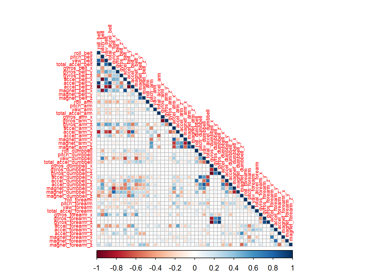
Due to the high correlation of some variables and considering the large number of variables, a principal component pre-processing will be performed. The procedure will retain 95% of the variability of the original variables.
#### Principal component pre-processing
preProc <- preProcess(training[, -nbrCol], method = "pca", thresh = 0.95)
#### Transform training dataset using PCA result (the outcome is not used)
trainingPC <- predict(preProc, training[, -nbrCol])
The processed dataset contains 25 predictors.
Method Selection
The random forest method has been selected since it is among the top performing algorithms. The random forest is also an appropriate model to perform classification of categorical outcomes. Model Training
A k-fold cross validation will be used during the training step. This method involves splitting the dataset into k-subsets. In this case, the number of folds has been set to 4.
#### Set the number of subsets for the k-fold cross validation
numberOfCrossValidation <- 4
#### The k-fold cross validation is set using "cv" option for method parameter
trainingControl <- trainControl(method = "cv", number = numberOfCrossValidation,
                                    allowParallel = TRUE)
#### Build a random forest model using k-fold cross validation
trainingModel <- train(training$classe ~ ., data=trainingPC, method="rf",
                        trControl = trainingControl)
trainingModel
## Random Forest
##
## 12757 samples
##    24 predictor
##     5 classes: 'A', 'B', 'C', 'D', 'E'
##
## No pre-processing
## Resampling: Cross-Validated (4 fold)
## Summary of sample sizes: 9568, 9568, 9568, 9567
## Resampling results across tuning parameters:
##
##   mtry  Accuracy   Kappa      Accuracy SD  Kappa SD
##    2    0.9636278  0.9539771  0.001932411  0.002432382
##   13    0.9572783  0.9459477  0.004400744  0.005556971
##   25    0.9531237  0.9406966  0.004704790  0.005940001
##
## Accuracy was used to select the optimal model using  the largest value.
## The final value used for the model was mtry = 2.

#### See the result for each submodel
plot(trainingModel)
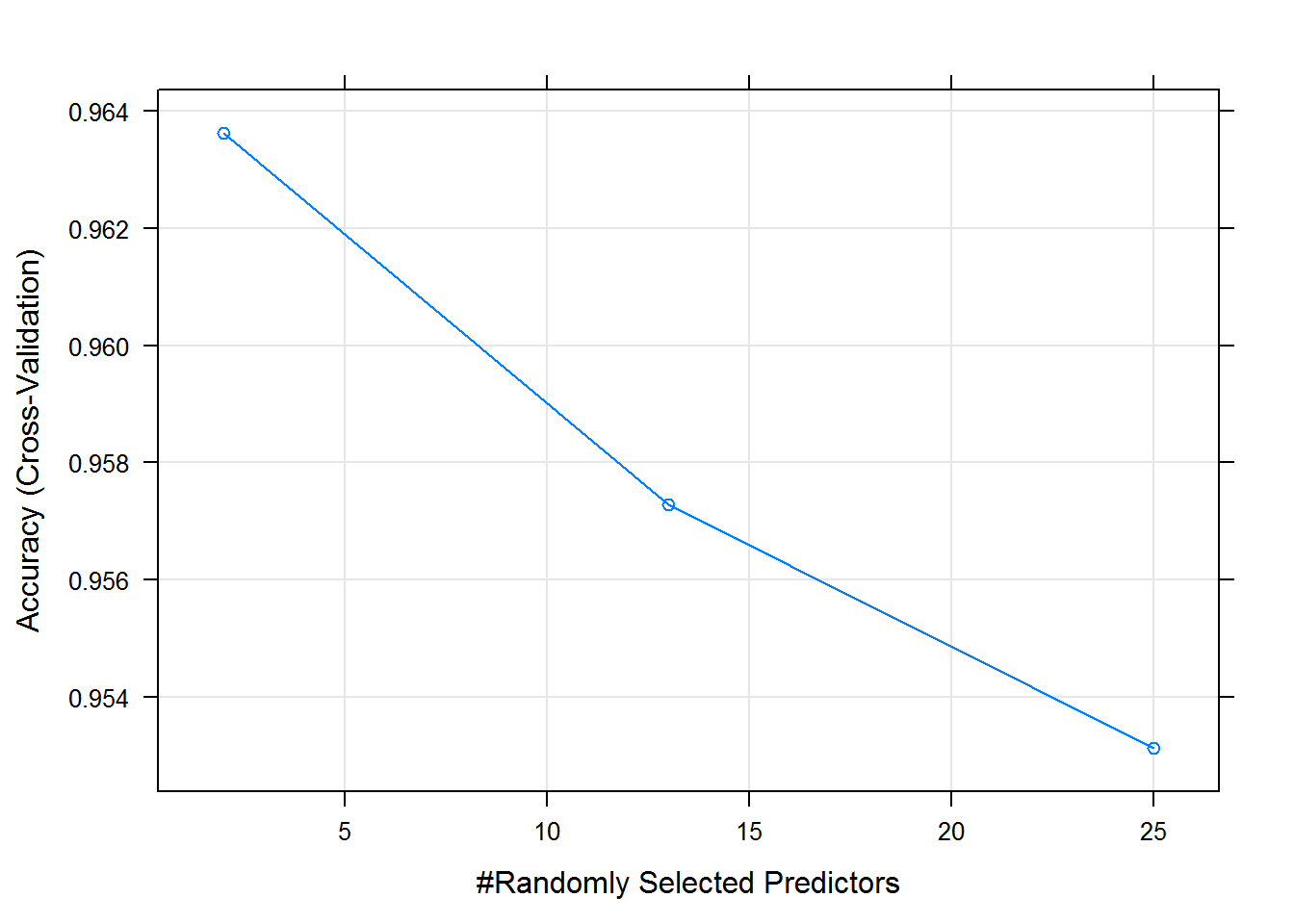
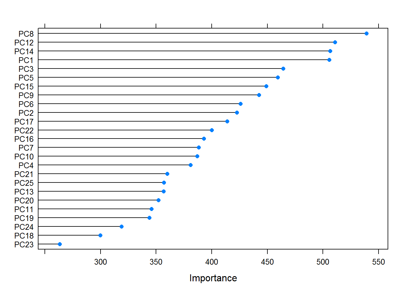
The training method used accuracy to select the optimal model. The importance of each variable in the final model can be visualized.
#### Calculate the importance of each variable in the model
mostImportantVar <- varImp(trainingModel, scale = FALSE)
plot(mostImportantVar)
Using the final model, the confusion matrix and statistics are extracted from the training dataset.
#### Calculate the confusion matrix using predicted versus real results
conf.matrix <- confusionMatrix(training$classe,
                                predict(trainingModel, trainingPC))
conf.matrix
## Confusion Matrix and Statistics
##
##           Reference
## Prediction    A    B    C    D    E
##          A 3627    0    0    0    0
##          B    0 2469    0    0    0
##          C    0    0 2225    0    0
##          D    0    0    0 2091    0
##          E    0    0    0    0 2345
##
## Overall Statistics
##
##                Accuracy : 1
##                  95% CI : (0.9997, 1)
##     No Information Rate : 0.2843
##     P-Value [Acc > NIR] : < 2.2e-16
##
##                   Kappa : 1
##  Mcnemar's Test P-Value : NA
##
## Statistics by Class:
##
##                      Class: A Class: B Class: C Class: D Class: E
## Sensitivity            1.0000   1.0000   1.0000   1.0000   1.0000
## Specificity            1.0000   1.0000   1.0000   1.0000   1.0000
## Pos Pred Value         1.0000   1.0000   1.0000   1.0000   1.0000
## Neg Pred Value         1.0000   1.0000   1.0000   1.0000   1.0000
## Prevalence             0.2843   0.1935   0.1744   0.1639   0.1838
## Detection Rate         0.2843   0.1935   0.1744   0.1639   0.1838
## Detection Prevalence   0.2843   0.1935   0.1744   0.1639   0.1838
## Balanced Accuracy      1.0000   1.0000   1.0000   1.0000   1.0000
Based on the accuracy results from the confusion matrix on the training data, the accuracy is 100%.
Out-of-sample Estimation
The testing test is used to estimate the out of sample error. The same cleaning steps must be applied to the testing dataset.
#### New testing dataset without variables with missing values
testing <- testing[, colnames(testing)[column_to_keep]]
#### The first 6 variables are removed from the testing dataset
testing <- testing[ , -c(1:6)]
#### Transform testing using PCA result
testingPC <- predict(preProc, testing[, -nbrCol])
Using the obtained model, the confusion matrix and statistics are extracted from the testing dataset.
#### Calculate the confusion matrix on the testing dataset
conf.matrix <- confusionMatrix(testing$classe,
                               predict(trainingModel, testingPC))
conf.matrix
## Confusion Matrix and Statistics
##
##           Reference
## Prediction    A    B    C    D    E
##          A 1927   10   13    1    2
##          B   21 1293   14    0    0
##          C    3   12 1172    9    1
##          D    1    0   36 1084    4
##          E    0    9   11    9 1233
##
## Overall Statistics
##
##                Accuracy : 0.9773
##                  95% CI : (0.9735, 0.9807)
##     No Information Rate : 0.2843
##     P-Value [Acc > NIR] : < 2.2e-16
##
##                   Kappa : 0.9713
##  Mcnemar's Test P-Value : NA
##
## Statistics by Class:
##
##                      Class: A Class: B Class: C Class: D Class: E
## Sensitivity            0.9872   0.9766   0.9406   0.9828   0.9944
## Specificity            0.9947   0.9937   0.9956   0.9929   0.9948
## Pos Pred Value         0.9867   0.9736   0.9791   0.9636   0.9770
## Neg Pred Value         0.9949   0.9944   0.9869   0.9967   0.9988
## Prevalence             0.2843   0.1929   0.1815   0.1607   0.1806
## Detection Rate         0.2807   0.1883   0.1707   0.1579   0.1796
## Detection Prevalence   0.2845   0.1934   0.1744   0.1639   0.1838
## Balanced Accuracy      0.9910   0.9851   0.9681   0.9878   0.9946
Based on the accuracy results from the confusion matrix on the training data, the accuracy is expected to be 97.73% and the out-of-sample error rate is expected to be 2.27%.
Prediction of 20 test cases
The model is used to predict 20 test cases.
#### URL for test cases
testingCasesURL <- "https://d396qusza40orc.cloudfront.net/predmachlearn/pml-testing.csv"
#### Load test cases
testingCases <- read.csv(url(testingCasesURL), row.names = 1)
#### Prepare test cases by keeping only pertinent variables
testingCases <- testingCases[, colnames(testingCases) %in% colnames(training)]
#### Transform test cases using PCA result
testingCasesPC <- predict(preProc, testingCases)
#### Predict classes using the model
predictedValues <- predict(trainingModel, testingCasesPC)
#### View predictions
predictedValues
##  [1] B A C A A E D B A A A C B A E E A B B B
## Levels: A B C D E
References
The data for this project come from this source: http://groupware.les.inf.puc-rio.br/har.
Ugulino, W.; Cardador, D.; Vega, K.; Velloso, E.; Milidiu, R.; Fuks, H. Wearable Computing: Accelerometers’ Data Classification of Body Postures and Movements. Proceedings of 21st Brazilian Symposium on Artificial Intelligence. Advances in Artificial Intelligence - SBIA 2012. In: Lecture Notes in Computer Science. , pp. 52-61. Curitiba, PR: Springer Berlin / Heidelberg, 2012. ISBN 978-3-642-34458-9. DOI: 10.1007/978-3-642-34459-6_6.